T-tests and Analysis of Variance (ANOVA)
Updated:
Overview
This notebook will analyze a fabricated dataset representing race and age of voters.
Tests used will include one-way ANOVA test, paired t-test, and Tukey's Range Test, starting with a baseline comparison before altering the data and moving on to the post hoc analyses.
Imports
%matplotlib inline
import numpy as np
import pandas as pd
import matplotlib.pyplot as plt
import scipy.stats as ss
from statsmodels.stats.multicomp import pairwise_tukeyhsd
Data
The data used in this notebook is randomly generated, following the procedures outlined in this blog post with minor alterations for segmentation purposes.
# Set a random state variable and assign it to scipy's random state
ss.poisson.random_state = rand = np.random.RandomState(404)
# Generate random data selected from a weighted distribution
races = ["asian", "black", "hispanic", "other", "white"]
voter_race = rand.choice(a=races, p=[0.05, 0.15, 0.25, 0.05, 0.5], size=1000)
voter_age = ss.poisson.rvs(loc=18, mu=30, size=1000)
white_ages = ss.poisson.rvs(loc=18, mu=32, size=1000) # increase the mean age of white voters

age_shift = np.where(voter_race=="white", white_ages, voter_age) # Swap in altered white ages
Exploratory Data Analysis
The data used in this notebook attempts to mock a racial distribution of a voter population sample. As it is artificially generated, no preprocessing is required.
# Group age data by race
voters = pd.DataFrame({"race":voter_race, "age":voter_age})
groups = voters.groupby("race").groups

# Perform the ANOVA
ss.f_oneway(*[voter_age[v] for v in groups.values()])
F_onewayResult(statistic=0.26737204976027656, pvalue=0.8990043212082999)
With a F-statistic of 0.2673 and a p-value of 0.899, the one-way ANOVA test provides a strong evidence that there is not a significant difference between means of each group. Since the data was all pulled from the same mock distribution, this is exactly what we would expect to see.
Modify Distribution and Reanalyze
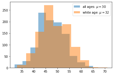
plt.hist(voter_age, alpha=0.5, label='all ages: $\mu=30$')
plt.hist(age_shift, alpha=0.5, label='white age: $\mu=32$')
plt.legend()
plt.show()

Now, we will be performing the same test on the modified dataset. Visually, we can already see how increasing the mean age of white voters effects the distribution.
# Group age data by race
voters_shift = pd.DataFrame({"race":voter_race, "age":age_shift})
groups_shift = voters_shift.groupby("race").groups

# Perform the ANOVA
ss.f_oneway(*[age_shift[v] for v in groups_shift.values()])
F_onewayResult(statistic=13.550717021659178, pvalue=9.24549061364278e-11)
After the change, the F-statistic is 13.55 and the p-value is 9.245e-11
A p-value of this size is many orders of magnitude smaller than p=0.05, a commonly used significance level. This serves as a very strong indication that there are indeed differences between the groups.
An F-statistic in the simplest sense is just the ratio of two variances. Building on this, an F-test is used for assessing whether the statistic follows an F-distribution under the null hypothesis.
A one-way ANOVA test uses F-tests as means to determine whether variance is due to differences within groups of data or differences between the groups. Put another way, a one-way ANOVA test assess whether variance between two or more (typically three or more) sample means is statistically significant.
# Get all unique racial pairings
race_pairs = [(races[r1], races[r2]) for r1 in range(4) for r2 in range(r1+1,5)]
# Conduct t-test on each pair for the altered data
for race1, race2 in race_pairs:
    print(race1, race2,'\t:', ss.ttest_ind(age_shift[groups_shift[race1]], age_shift[groups_shift[race2]]))
asian black 	: Ttest_indResult(statistic=0.5081230371721365, pvalue=0.6119242403088412)
asian hispanic 	: Ttest_indResult(statistic=0.6204493257066322, pvalue=0.5354223107249675)
asian other 	: Ttest_indResult(statistic=0.8804714769956019, pvalue=0.38034939855706185)
asian white 	: Ttest_indResult(statistic=-2.6589616806422485, pvalue=0.008072090696940136)
black hispanic 	: Ttest_indResult(statistic=0.12543582439538467, pvalue=0.9002425060815309)
black other 	: Ttest_indResult(statistic=0.6237279268453277, pvalue=0.5334896890146905)
black white 	: Ttest_indResult(statistic=-4.852584065988863, pvalue=1.5413623060362876e-06)
hispanic other 	: Ttest_indResult(statistic=0.5585844610829792, pvalue=0.5768434528987283)
hispanic white 	: Ttest_indResult(statistic=-6.0120762205487575, pvalue=2.89291138112763e-09)
other white 	: Ttest_indResult(statistic=-4.130139676281511, pvalue=4.195825609847373e-05)
# print the most likely candidates based on p-value and significance level
for race1, race2 in race_pairs:
    siglvl = 0.05
    result = ss.ttest_ind(age_shift[groups_shift[race1]], age_shift[groups_shift[race2]])
    if result.pvalue < siglvl:
        print(race1, race2,'\t:',result)
asian white 	: Ttest_indResult(statistic=-2.6589616806422485, pvalue=0.008072090696940136)
black white 	: Ttest_indResult(statistic=-4.852584065988863, pvalue=1.5413623060362876e-06)
hispanic white 	: Ttest_indResult(statistic=-6.0120762205487575, pvalue=2.89291138112763e-09)
other white 	: Ttest_indResult(statistic=-4.130139676281511, pvalue=4.195825609847373e-05)
With the one-way ANOVA test indicating a significant between groups did exist, conducting a pairwise t-test on each group pairing allows us to hone in on which group(s) stands out.
The p-values should be taken with a grain of salt, however, since as you increase the number of comparisons made, you as well introduce more opportunities for random chance to play a large factor. One of the simplest ways to address this is issue is with a Bonferroni correction.
A Bonferroni correction addresses the Multiple comparisons problem by simply dividing the starting significance level (e.g. p=0.05) by the number of comparisons made (in this case 10).
# endog = data, alpha = Significance level
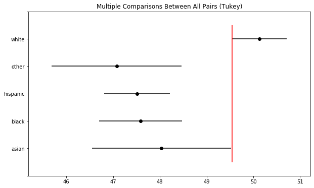
tukey2 = pairwise_tukeyhsd(endog=age_shift, groups=voter_race, alpha=0.05)

tukey2.plot_simultaneous() # Plot group confidence intervals
plt.vlines(x=49.55, ymin=-0.5, ymax=4.5, color="red")

tukey2.summary()
| group1 | group2 | meandiff | lower | upper | reject |
|---|---|---|---|---|---|
| asian | black | -0.4483 | -2.8332 | 1.9367 | False |
| asian | hispanic | -0.5205 | -2.757 | 1.7159 | False |
| asian | other | -0.9576 | -3.7303 | 1.8152 | False |
| asian | white | 2.0986 | -0.0352 | 4.2323 | False |
| black | hispanic | -0.0723 | -1.6735 | 1.529 | False |
| black | other | -0.5093 | -2.8007 | 1.7821 | False |
| black | white | 2.5468 | 1.0925 | 4.0012 | True |
| hispanic | other | -0.437 | -2.5734 | 1.6994 | False |
| hispanic | white | 2.6191 | 1.4238 | 3.8144 | True |
| other | white | 3.0561 | 1.0275 | 5.0847 | True |

Tukey's test is more exacting in the way that it approaches the Multiple comparisons problem. Rather than conducting pairwise t-tests and adjusting the significance level to compensate, Tukey's test, in effect, combines t-tests with an adjustment made to correct for the family-wise error rate.
Tukey's test is not the most precise for all cases but works quite well when confidence intervals are needed or sample sizes are unequal.
Conclusions
This note demonstrated the use of:
- one-way ANOVA test
- pairwise t-tests
- Tukey's range test
on a generated dataset representing fictitious voter demographics.
Future works could involve the use of a real vote demographic dataset, as opposed to a mocked up one, exploring other methods of dealing with the multiple comparison problem (e.g. Scheffé's method, Newman–Keuls method), and potentially using other variants of ANOVA tests.
References
Text:
- http://hamelg.blogspot.com/2015/11/python-for-data-analysis-part-16_23.html
- http://statisticsbyjim.com/anova/f-tests-anova/
- https://www.statisticshowto.datasciencecentral.com/probability-and-statistics/f-statistic-value-test/#FandP
- http://blog.minitab.com/blog/adventures-in-statistics-2/understanding-analysis-of-variance-anova-and-the-f-test
- https://en.wikipedia.org/wiki/One-way_analysis_of_variance
- https://en.wikipedia.org/wiki/F-test
Code:
Tags: ANOVA, python, statistics, ttests, voting
Categories: python, statistics