Dimensionality Reduction and Feature Analysis
Updated:
Overview
This notebook will take a second look at the 2016 Kaggle Caravan Insurance Challenge.
This time around, EDA will include: * Stepwise feature selection based on p-values * Principal component analysis * t-SNE (optional) * UMAP (optional)
As well as modeling with: * Recursive feature elimination * Feature importance analysis
performed on a Logistic Regressor and Random Forest Classifier where applicable.
Imports
library(tidyverse)
library(caret)
library(MASS)
library(SignifReg) # p-value stepwise feature selection
library(factoextra) # pretty PCA plot
# setup for parallel processing
library(doParallel)
cl <- makePSOCKcluster(8)
registerDoParallel(cl)Data
The dataset used is from the CoIL Challenge 2000 datamining competition. It may be obtained from: https://www.kaggle.com/uciml/caravan-insurance-challenge
It contains information on customers of an insurance company. The data consists of 86 variables and includes product usage data and socio-demographic data derived from zip area codes.
A description of each variable may be found at the link in this cell listed above
The variable descriptions are quite important as it appears as though the variable names themselves are abbreviated in Dutch. One helpful pattern to notice is the letters that variables begin with:
- M - primary demographics?, no guess for abbreviation
- A - numbers, likely for dutch word aantal
- P - percents, likely for dutch word procent
Acknowledgements:
P. van der Putten and M. van Someren (eds) . CoIL Challenge 2000: The Insurance Company Case. Published by Sentient Machine Research, Amsterdam. Also a Leiden Institute of Advanced Computer Science Technical Report 2000-09. June 22, 2000.
head(cic <- read.csv('data/caravan-insurance-challenge.csv'))Exploratory Data Analysis
No NA values, all variables are type of int64. The data is peculiar in that every numeric value stands for an attribute of a person. Even variables that could be continuous, such as income, have been binned. In this sense, this dataset is entirely comprised of Categorical and Ordinal values. Other than potential collinearity between percentage and range values, the data is mostly clean.
In contrast with the previous notebook, this time around we will not try and mimic competition settings and instead just use the whole dataset throughout since we are more focused on describing the data rather than predicting.
cic_data <- subset(cic, select=-c(ORIGIN))Stepwise Feature Selection
We will be using the SignifReg package to carryout both
foward and backward stepwise feature selection. This process iteratively
builds a linear model by examining how the model responds to
modifications in the predictor variable set. The parameter
alpha serves as our threshold p-value,
correction specifies the method for adjusting p-value
scoring to help mitigate the Multiple
comparisons problem.
In the forward case, the model is built up one variable at a time, each step selecting the variable whose addition resulted in the lowest overall p-value. The process continues until there are no possible additions that can be made that satisfy the p-value threshold criterion.
When the backward method is used, the model begins with the full set
of predictor variables then, one by one, begins reducing the feature set
by removing the variable with the highest p-value. The process is
repeated until there are no variables left whose p-value is greater than
the alpha threshold criterion.
Using p-values
# Forward pass
step.pvmodel.fwd <- SignifReg(lm(CARAVAN ~ ., data=cic_data),
                    alpha=0.05, direction="forward",
                    criterion="p-value",adjust.method="fdr", trace = FALSE)

summary(step.pvmodel.fwd)
##
## Call:
## lm(formula = CARAVAN ~ ., data = cic_data)
##
## Residuals:
## Min 1Q Median 3Q Max
## -0.59686 -0.08677 -0.04731 -0.00935 1.04207
##
## Coefficients:
## Estimate Std. Error t value Pr(>|t|)
## (Intercept) 0.5783847 0.3591997 1.610 0.107386
## MOSTYPE 0.0017034 0.0017257 0.987 0.323620
## MAANTHUI -0.0030908 0.0058102 -0.532 0.594765
## MGEMOMV 0.0018860 0.0055376 0.341 0.733425
## MGEMLEEF 0.0081546 0.0038467 2.120 0.034037 *
## MOSHOOFD -0.0058416 0.0077350 -0.755 0.450137
## MGODRK -0.0011922 0.0043126 -0.276 0.782208
## MGODPR 0.0016262 0.0046996 0.346 0.729335
## MGODOV 0.0033623 0.0042110 0.798 0.424622
## MGODGE -0.0006484 0.0045023 -0.144 0.885486
## MRELGE 0.0073003 0.0058266 1.253 0.210267
## MRELSA 0.0017438 0.0055644 0.313 0.754002
## MRELOV 0.0058132 0.0058812 0.988 0.322965
## MFALLEEN -0.0068756 0.0049762 -1.382 0.167098
## MFGEKIND -0.0076840 0.0051113 -1.503 0.132780
## MFWEKIND -0.0055513 0.0053244 -1.043 0.297159
## MOPLHOOG 0.0049231 0.0052219 0.943 0.345822
## MOPLMIDD -0.0014082 0.0054568 -0.258 0.796371
## MOPLLAAG -0.0058663 0.0056023 -1.047 0.295063
## MBERHOOG -0.0013785 0.0034649 -0.398 0.690743
## MBERZELF 0.0031623 0.0040297 0.785 0.432620
## MBERBOER -0.0105737 0.0038122 -2.774 0.005554 **
## MBERMIDD 0.0019283 0.0034542 0.558 0.576681
## MBERARBG -0.0005993 0.0034539 -0.174 0.862241
## MBERARBO -0.0002782 0.0034164 -0.081 0.935095
## MSKA -0.0022806 0.0040211 -0.567 0.570614
## MSKB1 -0.0039062 0.0038612 -1.012 0.311728
## MSKB2 -0.0033504 0.0034535 -0.970 0.331988
## MSKC -0.0019335 0.0037918 -0.510 0.610116
## MSKD -0.0005069 0.0036463 -0.139 0.889447
## MHHUUR -0.0238305 0.0307539 -0.775 0.438432
## MHKOOP -0.0216805 0.0307182 -0.706 0.480337
## MAUT1 0.0116511 0.0057850 2.014 0.044037 *
## MAUT2 0.0080192 0.0052851 1.517 0.129216
## MAUT0 0.0077346 0.0055589 1.391 0.164140
## MZFONDS -0.0589186 0.0369015 -1.597 0.110377
## MZPART -0.0600217 0.0368420 -1.629 0.103311
## MINKM30 0.0055613 0.0039235 1.417 0.156386
## MINK3045 0.0050760 0.0037877 1.340 0.180234
## MINK4575 0.0034224 0.0038337 0.893 0.372026
## MINK7512 0.0013611 0.0040272 0.338 0.735389
## MINK123M -0.0130376 0.0053561 -2.434 0.014944 *
## MINKGEM 0.0076177 0.0035222 2.163 0.030583 *
## MKOOPKLA 0.0043055 0.0017605 2.446 0.014477 *
## PWAPART 0.0352508 0.0126978 2.776 0.005511 **
## PWABEDR -0.0112595 0.0165518 -0.680 0.496358
## PWALAND -0.0149981 0.0263041 -0.570 0.568568
## PPERSAUT 0.0094506 0.0019336 4.887 1.04e-06 ***
## PBESAUT 0.0009264 0.0097120 0.095 0.924010
## PMOTSCO -0.0076253 0.0068607 -1.111 0.266405
## PVRAAUT -0.0180541 0.0231880 -0.779 0.436237
## PAANHANG 0.0335455 0.0432778 0.775 0.438287
## PTRACTOR 0.0066051 0.0099400 0.664 0.506387
## PWERKT -0.0165037 0.0278616 -0.592 0.553633
## PBROM 0.0048050 0.0114610 0.419 0.675042
## PLEVEN -0.0114336 0.0049549 -2.308 0.021047 *
## PPERSONG -0.0158814 0.0285207 -0.557 0.577652
## PGEZONG 0.1843040 0.0547670 3.365 0.000768 ***
## PWAOREG 0.0290693 0.0222813 1.305 0.192043
## PBRAND 0.0148741 0.0027718 5.366 8.22e-08 ***
## PZEILPL -0.0480886 0.1239554 -0.388 0.698061
## PPLEZIER -0.0011871 0.0216523 -0.055 0.956279
## PFIETS -0.0179992 0.0413143 -0.436 0.663090
## PINBOED -0.0376564 0.0220828 -1.705 0.088182 .
## PBYSTAND 0.0351617 0.0224860 1.564 0.117916
## AWAPART -0.0501723 0.0247235 -2.029 0.042451 *
## AWABEDR 0.0202559 0.0451784 0.448 0.653908
## AWALAND -0.0095720 0.0925739 -0.103 0.917649
## APERSAUT -0.0008198 0.0092918 -0.088 0.929698
## ABESAUT -0.0287920 0.0436043 -0.660 0.509076
## AMOTSCO 0.0171126 0.0272229 0.629 0.529619
## AVRAAUT 0.0438739 0.0807139 0.544 0.586748
## AAANHANG -0.0352543 0.0749002 -0.471 0.637877
## ATRACTOR -0.0226762 0.0233543 -0.971 0.331590
## AWERKT 0.0219802 0.0561490 0.391 0.695465
## ABROM -0.0110523 0.0346947 -0.319 0.750068
## ALEVEN 0.0340398 0.0116835 2.914 0.003582 **
## APERSONG 0.0193591 0.0793315 0.244 0.807214
## AGEZONG -0.3776992 0.1322457 -2.856 0.004299 **
## AWAOREG -0.1183782 0.1172535 -1.010 0.312716
## ABRAND -0.0249035 0.0089953 -2.769 0.005642 **
## AZEILPL 0.3166501 0.2350619 1.347 0.177982
## APLEZIER 0.2220372 0.0672979 3.299 0.000973 ***
## AFIETS 0.0328653 0.0310300 1.059 0.289560
## AINBOED 0.0658758 0.0506052 1.302 0.193029
## ABYSTAND -0.0638010 0.0758703 -0.841 0.400413
## ---
## Signif. codes: 0 '***' 0.001 '**' 0.01 '*' 0.05 '.' 0.1 ' ' 1
##
## Residual standard error: 0.2303 on 9736 degrees of freedom
## Multiple R-squared: 0.06284, Adjusted R-squared: 0.05465
## F-statistic: 7.68 on 85 and 9736 DF, p-value: < 2.2e-16# Reduce down to best/worst to save time
sumfwd <- summary(step.pvmodel.fwd)
pvals <- sumfwd$coefficients[,4]
feat_extremes <- pvals[pvals < 0.1 | pvals > 0.9] %>% names() %>% .[. != "(Intercept)"]
fmla <- as.formula(paste("CARAVAN ~ ", paste(feat_extremes, collapse= "+")))
fit_extreme <- lm(fmla, data = cic_data)
fit_extreme##
## Call:
## lm(formula = fmla, data = cic_data)
##
## Coefficients:
## (Intercept) MGEMLEEF MBERBOER MBERARBO MAUT1 MINK123M
## -0.0763392 0.0056824 -0.0102959 -0.0020071 0.0040516 -0.0130215
## MINKGEM MKOOPKLA PWAPART PPERSAUT PBESAUT PLEVEN
## 0.0089861 0.0059283 0.0367790 0.0090817 -0.0055774 -0.0114734
## PGEZONG PBRAND PPLEZIER PINBOED AWAPART AWALAND
## 0.1808067 0.0157212 0.0064432 -0.0096923 -0.0524946 -0.0688962
## APERSAUT ALEVEN AGEZONG ABRAND APLEZIER
## 0.0004565 0.0344180 -0.3590850 -0.0269530 0.2136198# Backward pass
step.pvmodel.bkwd <- SignifReg(fit = fit_extreme,
alpha=0.05, direction="backward",
criterion="p-value", adjust.method="fdr", trace = FALSE)
summary(step.pvmodel.bkwd)##
## Call:
## lm(formula = CARAVAN ~ MBERBOER + MBERARBO + MINK123M + MKOOPKLA +
## PWAPART + PGEZONG + PBRAND + AGEZONG, data = cic_data)
##
## Residuals:
## Min 1Q Median 3Q Max
## -0.33462 -0.08085 -0.05370 -0.02634 1.00847
##
## Coefficients:
## Estimate Std. Error t value Pr(>|t|)
## (Intercept) 0.009551 0.008330 1.147 0.251577
## MBERBOER -0.011691 0.002191 -5.336 9.73e-08 ***
## MBERARBO -0.003975 0.001506 -2.640 0.008314 **
## MINK123M -0.010126 0.004279 -2.366 0.017978 *
## MKOOPKLA 0.009571 0.001290 7.420 1.27e-13 ***
## PWAPART 0.015597 0.002844 5.485 4.24e-08 ***
## PGEZONG 0.191883 0.055175 3.478 0.000508 ***
## PBRAND 0.007772 0.001455 5.343 9.36e-08 ***
## AGEZONG -0.373704 0.132862 -2.813 0.004922 **
## ---
## Signif. codes: 0 '***' 0.001 '**' 0.01 '*' 0.05 '.' 0.1 ' ' 1
##
## Residual standard error: 0.2337 on 9813 degrees of freedom
## Multiple R-squared: 0.02724, Adjusted R-squared: 0.02644
## F-statistic: 34.34 on 8 and 9813 DF, p-value: < 2.2e-16There is a very good reason this p-value based approach is not
included in more common packages like stats or
MASS, the results can often be very miss
leading. If a stepwise feature selection approach is used, it is far
better to use a different scoring criterion,such as AIC, or Mallows’ Cp.
However,even using these feature selection criteria, it is still prone
to overfitting and can provide biased, if not completely flawed results,
especially in the presence of multicollinearity. By using p-values as
our criterion, not only do we have the aforementioned issues, now we
introduce the Multiple
Comparisons Problem, so it stands to reason that the features
selected by this method disagree more so than the others.
Using AIC
full_model <- lm(CARAVAN ~., data = cic_data)
step.aicmodel.both <- stepAIC(full_model, direction = "both", trace = FALSE, steps=10)
Using AIC as the evaluating metric rather than p-value allows us to use a bidirectional approach through the feature set, providing a more thoroughly vetted set of predictor variables.
summary(step.aicmodel.both)##
## Call:
## lm(formula = CARAVAN ~ MOSTYPE + MAANTHUI + MGEMOMV + MGEMLEEF +
## MOSHOOFD + MGODPR + MGODOV + MRELGE + MRELSA + MRELOV + MFALLEEN +
## MFGEKIND + MFWEKIND + MOPLHOOG + MOPLMIDD + MOPLLAAG + MBERHOOG +
## MBERZELF + MBERBOER + MBERMIDD + MSKA + MSKB1 + MSKB2 + MSKC +
## MHHUUR + MHKOOP + MAUT1 + MAUT2 + MAUT0 + MZFONDS + MZPART +
## MINKM30 + MINK3045 + MINK4575 + MINK7512 + MINK123M + MINKGEM +
## MKOOPKLA + PWAPART + PWABEDR + PWALAND + PPERSAUT + PMOTSCO +
## PVRAAUT + PAANHANG + PTRACTOR + PWERKT + PBROM + PLEVEN +
## PPERSONG + PGEZONG + PWAOREG + PBRAND + PZEILPL + PFIETS +
## PINBOED + PBYSTAND + AWAPART + AWABEDR + ABESAUT + AMOTSCO +
## AVRAAUT + AAANHANG + ATRACTOR + AWERKT + ABROM + ALEVEN +
## AGEZONG + AWAOREG + ABRAND + AZEILPL + APLEZIER + AFIETS +
## AINBOED + ABYSTAND, data = cic_data)
##
## Residuals:
## Min 1Q Median 3Q Max
## -0.59327 -0.08685 -0.04757 -0.00938 1.04216
##
## Coefficients:
## Estimate Std. Error t value Pr(>|t|)
## (Intercept) 0.5724299 0.3570989 1.603 0.108967
## MOSTYPE 0.0016864 0.0017196 0.981 0.326764
## MAANTHUI -0.0030670 0.0057924 -0.529 0.596476
## MGEMOMV 0.0019597 0.0055155 0.355 0.722372
## MGEMLEEF 0.0081143 0.0038394 2.113 0.034588 *
## MOSHOOFD -0.0057459 0.0077099 -0.745 0.456132
## MGODPR 0.0024028 0.0015469 1.553 0.120392
## MGODOV 0.0039067 0.0025186 1.551 0.120896
## MRELGE 0.0069933 0.0056925 1.228 0.219289
## MRELSA 0.0014456 0.0054296 0.266 0.790054
## MRELOV 0.0055055 0.0057076 0.965 0.334774
## MFALLEEN -0.0069371 0.0049260 -1.408 0.159089
## MFGEKIND -0.0077321 0.0050739 -1.524 0.127565
## MFWEKIND -0.0056485 0.0052725 -1.071 0.284052
## MOPLHOOG 0.0046980 0.0051598 0.911 0.362578
## MOPLMIDD -0.0016588 0.0053805 -0.308 0.757868
## MOPLLAAG -0.0061594 0.0054637 -1.127 0.259636
## MBERHOOG -0.0010733 0.0024275 -0.442 0.658383
## MBERZELF 0.0033968 0.0035678 0.952 0.341090
## MBERBOER -0.0102245 0.0029125 -3.511 0.000449 ***
## MBERMIDD 0.0023020 0.0018508 1.244 0.213612
## MSKA -0.0019936 0.0035439 -0.563 0.573766
## MSKB1 -0.0036625 0.0030206 -1.213 0.225343
## MSKB2 -0.0031161 0.0025099 -1.242 0.214439
## MSKC -0.0017154 0.0023368 -0.734 0.462925
## MHHUUR -0.0235186 0.0305618 -0.770 0.441589
## MHKOOP -0.0214107 0.0305246 -0.701 0.483055
## MAUT1 0.0113245 0.0056760 1.995 0.046055 *
## MAUT2 0.0077296 0.0051937 1.488 0.136716
## MAUT0 0.0073747 0.0054296 1.358 0.174414
## MZFONDS -0.0588420 0.0367675 -1.600 0.109546
## MZPART -0.0599352 0.0367201 -1.632 0.102666
## MINKM30 0.0053045 0.0038309 1.385 0.166194
## MINK3045 0.0048150 0.0036846 1.307 0.191324
## MINK4575 0.0031321 0.0037030 0.846 0.397675
## MINK7512 0.0010579 0.0039042 0.271 0.786433
## MINK123M -0.0134459 0.0052262 -2.573 0.010103 *
## MINKGEM 0.0076835 0.0035113 2.188 0.028679 *
## MKOOPKLA 0.0043447 0.0017496 2.483 0.013037 *
## PWAPART 0.0351616 0.0126789 2.773 0.005561 **
## PWABEDR -0.0110759 0.0165222 -0.670 0.502640
## PWALAND -0.0176335 0.0057591 -3.062 0.002206 **
## PPERSAUT 0.0093065 0.0008407 11.070 < 2e-16 ***
## PMOTSCO -0.0076492 0.0068517 -1.116 0.264284
## PVRAAUT -0.0178551 0.0230878 -0.773 0.439329
## PAANHANG 0.0334802 0.0431691 0.776 0.438029
## PTRACTOR 0.0065646 0.0099107 0.662 0.507745
## PWERKT -0.0156597 0.0268700 -0.583 0.560046
## PBROM 0.0047397 0.0114522 0.414 0.678980
## PLEVEN -0.0113667 0.0049440 -2.299 0.021521 *
## PPERSONG -0.0095662 0.0124760 -0.767 0.443241
## PGEZONG 0.1844539 0.0546213 3.377 0.000736 ***
## PWAOREG 0.0292366 0.0222448 1.314 0.188771
## PBRAND 0.0148643 0.0027664 5.373 7.92e-08 ***
## PZEILPL -0.0480655 0.1229430 -0.391 0.695837
## PFIETS -0.0180838 0.0412741 -0.438 0.661296
## PINBOED -0.0378742 0.0220526 -1.717 0.085929 .
## PBYSTAND 0.0354185 0.0224146 1.580 0.114103
## AWAPART -0.0500644 0.0246897 -2.028 0.042613 *
## AWABEDR 0.0200906 0.0451182 0.445 0.656122
## ABESAUT -0.0251562 0.0198435 -1.268 0.204925
## AMOTSCO 0.0171959 0.0271983 0.632 0.527243
## AVRAAUT 0.0430724 0.0802005 0.537 0.591239
## AAANHANG -0.0352425 0.0747284 -0.472 0.637218
## ATRACTOR -0.0226610 0.0232812 -0.973 0.330398
## AWERKT 0.0197019 0.0534293 0.369 0.712325
## ABROM -0.0108239 0.0346618 -0.312 0.754841
## ALEVEN 0.0339156 0.0116517 2.911 0.003613 **
## AGEZONG -0.3782742 0.1317989 -2.870 0.004112 **
## AWAOREG -0.1188004 0.1171097 -1.014 0.310399
## ABRAND -0.0248331 0.0089837 -2.764 0.005717 **
## AZEILPL 0.3163373 0.2324447 1.361 0.173572
## APLEZIER 0.2186388 0.0300053 7.287 3.42e-13 ***
## AFIETS 0.0330478 0.0310011 1.066 0.286442
## AINBOED 0.0664611 0.0504942 1.316 0.188133
## ABYSTAND -0.0646050 0.0755661 -0.855 0.392602
## ---
## Signif. codes: 0 '***' 0.001 '**' 0.01 '*' 0.05 '.' 0.1 ' ' 1
##
## Residual standard error: 0.2302 on 9746 degrees of freedom
## Multiple R-squared: 0.06281, Adjusted R-squared: 0.0556
## F-statistic: 8.709 on 75 and 9746 DF, p-value: < 2.2e-16A quick summary shows how this method chose to keep far more values than the stepwise p-value approach.
(feats.pv <- intersect(names(step.pvmodel.bkwd$coefficients), names(step.pvmodel.fwd$coefficients)))## [1] "(Intercept)" "MBERBOER" "MBERARBO" "MINK123M" "MKOOPKLA"
## [6] "PWAPART" "PGEZONG" "PBRAND" "AGEZONG"feats.shared <- intersect(names(step.aicmodel.both$coefficients),feats.pv)
length(feats.shared)## [1] 8(feats.aic <- setdiff(names(step.aicmodel.both$coefficients),feats.pv))## [1] "MOSTYPE" "MAANTHUI" "MGEMOMV" "MGEMLEEF" "MOSHOOFD" "MGODPR"
## [7] "MGODOV" "MRELGE" "MRELSA" "MRELOV" "MFALLEEN" "MFGEKIND"
## [13] "MFWEKIND" "MOPLHOOG" "MOPLMIDD" "MOPLLAAG" "MBERHOOG" "MBERZELF"
## [19] "MBERMIDD" "MSKA" "MSKB1" "MSKB2" "MSKC" "MHHUUR"
## [25] "MHKOOP" "MAUT1" "MAUT2" "MAUT0" "MZFONDS" "MZPART"
## [31] "MINKM30" "MINK3045" "MINK4575" "MINK7512" "MINKGEM" "PWABEDR"
## [37] "PWALAND" "PPERSAUT" "PMOTSCO" "PVRAAUT" "PAANHANG" "PTRACTOR"
## [43] "PWERKT" "PBROM" "PLEVEN" "PPERSONG" "PWAOREG" "PZEILPL"
## [49] "PFIETS" "PINBOED" "PBYSTAND" "AWAPART" "AWABEDR" "ABESAUT"
## [55] "AMOTSCO" "AVRAAUT" "AAANHANG" "ATRACTOR" "AWERKT" "ABROM"
## [61] "ALEVEN" "AWAOREG" "ABRAND" "AZEILPL" "APLEZIER" "AFIETS"
## [67] "AINBOED" "ABYSTAND"length(feats.aic )## [1] 68There were a total of 15 shared features identified as a statistically significant using the stepwise p-value approach. In addition to these variables, the bidirectional AIC approach included 20 other features that did not meet the 0.05 p-value threshold, but did meet the AIC statistic.
Principal Components Analysis (PCA)
In contrast the previous stepwise approach to feature selection, PCA does not filter out variables based on a metric, but rather, attempts to combine them in such a manner that the conglomerate variables explain the largest amount of variance.
In using PCA, we are not attempting reduce the overall feature set, we are reducing the dimensionality of the dataset. In this example, the coil2k dataset has 86 columns (85 predictors + 1 response), plotting this many features in 2 or even 3 dimensional space is simply not practically possible. With PCA, we exact useful interactions (Eigenvectors) that can be plotted in these lower dimensional spaces.
cic.pca <- prcomp(~ . -CARAVAN, data=cic_data, center = TRUE, scale. = TRUE)
(spca <- summary(cic.pca))
## Importance of components:
## PC1 PC2 PC3 PC4 PC5 PC6 PC7
## Standard deviation 3.0627 2.21527 1.99574 1.82836 1.71113 1.6259 1.50398
## Proportion of Variance 0.1104 0.05773 0.04686 0.03933 0.03445 0.0311 0.02661
## Cumulative Proportion 0.1104 0.16809 0.21495 0.25428 0.28872 0.3198 0.34643
## PC8 PC9 PC10 PC11 PC12 PC13 PC14
## Standard deviation 1.49545 1.46284 1.4520 1.41766 1.39902 1.38336 1.37946
## Proportion of Variance 0.02631 0.02518 0.0248 0.02364 0.02303 0.02251 0.02239
## Cumulative Proportion 0.37274 0.39792 0.4227 0.44637 0.46939 0.49191 0.51430
## PC15 PC16 PC17 PC18 PC19 PC20 PC21
## Standard deviation 1.36700 1.35872 1.34751 1.34003 1.31395 1.29922 1.28370
## Proportion of Variance 0.02198 0.02172 0.02136 0.02113 0.02031 0.01986 0.01939
## Cumulative Proportion 0.53628 0.55800 0.57936 0.60049 0.62080 0.64066 0.66004
## PC22 PC23 PC24 PC25 PC26 PC27 PC28
## Standard deviation 1.27285 1.24669 1.2056 1.19470 1.17662 1.14819 1.12893
## Proportion of Variance 0.01906 0.01829 0.0171 0.01679 0.01629 0.01551 0.01499
## Cumulative Proportion 0.67910 0.69739 0.7145 0.73128 0.74757 0.76308 0.77807
## PC29 PC30 PC31 PC32 PC33 PC34 PC35
## Standard deviation 1.09927 1.09201 1.06524 1.02851 0.98657 0.97396 0.93596
## Proportion of Variance 0.01422 0.01403 0.01335 0.01245 0.01145 0.01116 0.01031
## Cumulative Proportion 0.79229 0.80632 0.81967 0.83212 0.84357 0.85473 0.86503
## PC36 PC37 PC38 PC39 PC40 PC41 PC42
## Standard deviation 0.92309 0.90232 0.89200 0.8793 0.86819 0.84464 0.82404
## Proportion of Variance 0.01002 0.00958 0.00936 0.0091 0.00887 0.00839 0.00799
## Cumulative Proportion 0.87506 0.88464 0.89400 0.9031 0.91196 0.92035 0.92834
## PC43 PC44 PC45 PC46 PC47 PC48 PC49
## Standard deviation 0.78679 0.77184 0.74966 0.68517 0.68063 0.61773 0.58161
## Proportion of Variance 0.00728 0.00701 0.00661 0.00552 0.00545 0.00449 0.00398
## Cumulative Proportion 0.93562 0.94263 0.94924 0.95477 0.96022 0.96471 0.96869
## PC50 PC51 PC52 PC53 PC54 PC55 PC56
## Standard deviation 0.56714 0.44414 0.41342 0.38276 0.3802 0.36606 0.35593
## Proportion of Variance 0.00378 0.00232 0.00201 0.00172 0.0017 0.00158 0.00149
## Cumulative Proportion 0.97247 0.97479 0.97680 0.97853 0.9802 0.98180 0.98329
## PC57 PC58 PC59 PC60 PC61 PC62 PC63
## Standard deviation 0.33961 0.32794 0.32222 0.31307 0.30212 0.29990 0.28570
## Proportion of Variance 0.00136 0.00127 0.00122 0.00115 0.00107 0.00106 0.00096
## Cumulative Proportion 0.98465 0.98591 0.98714 0.98829 0.98936 0.99042 0.99138
## PC64 PC65 PC66 PC67 PC68 PC69 PC70
## Standard deviation 0.27841 0.27363 0.25798 0.24969 0.23323 0.20981 0.19857
## Proportion of Variance 0.00091 0.00088 0.00078 0.00073 0.00064 0.00052 0.00046
## Cumulative Proportion 0.99229 0.99317 0.99396 0.99469 0.99533 0.99585 0.99631
## PC71 PC72 PC73 PC74 PC75 PC76 PC77
## Standard deviation 0.19012 0.18577 0.17967 0.17695 0.16922 0.16705 0.16225
## Proportion of Variance 0.00043 0.00041 0.00038 0.00037 0.00034 0.00033 0.00031
## Cumulative Proportion 0.99674 0.99714 0.99752 0.99789 0.99823 0.99856 0.99887
## PC78 PC79 PC80 PC81 PC82 PC83 PC84
## Standard deviation 0.14070 0.13942 0.13586 0.1305 0.12348 0.07384 0.02532
## Proportion of Variance 0.00023 0.00023 0.00022 0.0002 0.00018 0.00006 0.00001
## Cumulative Proportion 0.99910 0.99933 0.99955 0.9998 0.99993 0.99999 1.00000
## PC85
## Standard deviation 0.01621
## Proportion of Variance 0.00000
## Cumulative Proportion 1.00000Looking the Cumulative Proportion of variance explained, it does not look like this dataset will provide a great deal of insight from PCA plotting. Only 16.8% of overall variance is explained by the second variable, ideally we’d like that to quite a bit larger.
spca$importance[3,] %>% enframe(value = "var_explained") %>%
  ggplot(aes(x=1:85, y=var_explained)) +
  geom_line() +
  geom_hline(aes(yintercept = .90), color="red", linetype=2) +
  scale_x_continuous(breaks = seq(0,85,5)) +
  xlab("n_components") +
  ylab("variance explained") +
  ggtitle("Cumulative Variance Explained")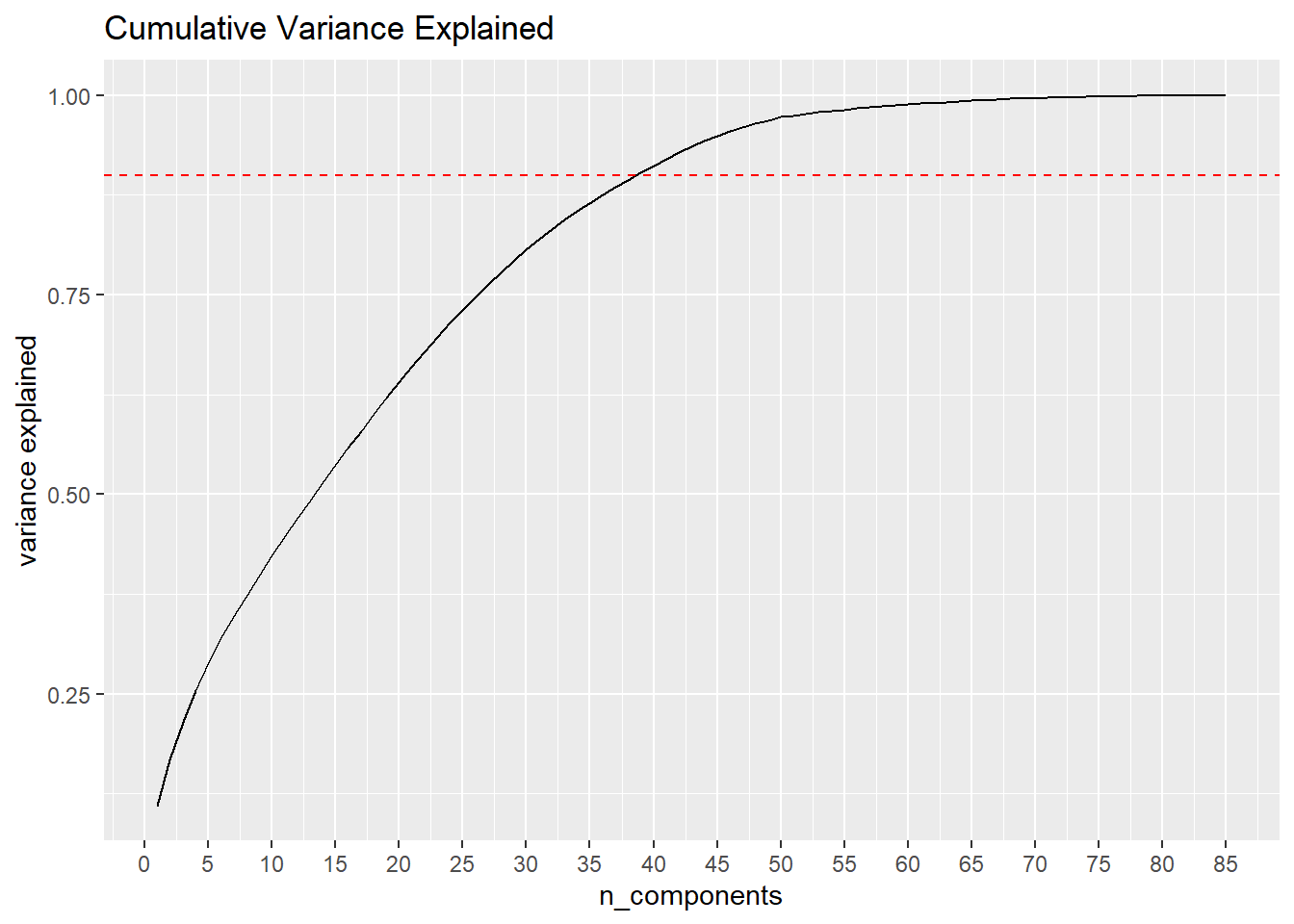
However, after only 39 components we are able to account for 90% of total variance, and by 62 components we reach 99%. This may be an indication that some variables in the dataset are providing little aditional information to the analysis.
fviz_pca_ind(cic.pca, geom = "point",
             pointshape = 21,
             fill.ind = as.factor(cic_data$CARAVAN),
             palette = "jco",
             addEllipses = TRUE,
             repel = TRUE,
             legend.title = "CARAVAN") +
  ggtitle("PCA-plot full feature set") +
  theme(plot.title = element_text(hjust = 0.5))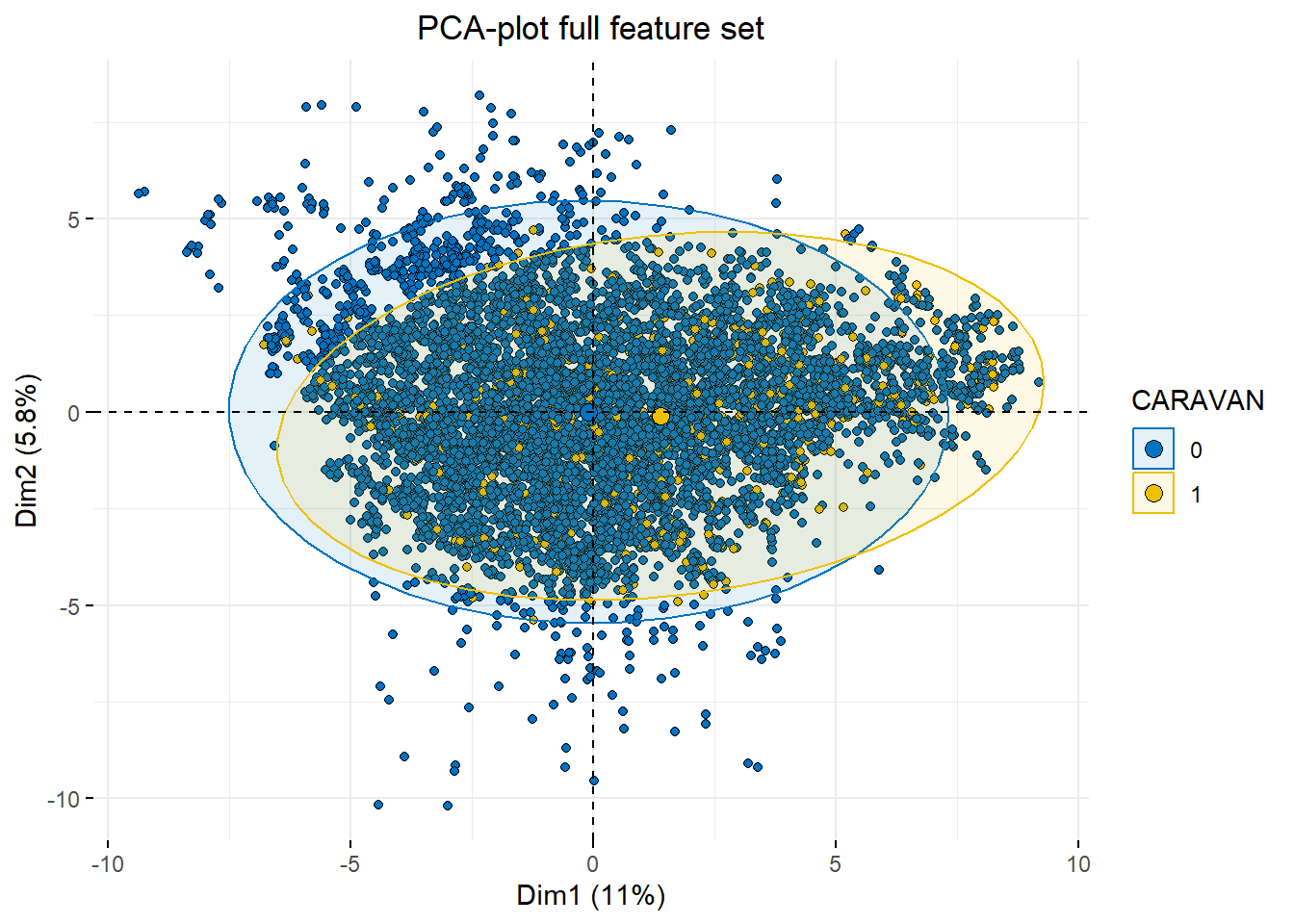
Using all 80 features makes our illustration a cluttered, overlaping mess, instead, let’s reduce the feature set to the 15 common features between the various methods of stepwise feature selection.
cic_sm <- cic_data[feats.shared[2:length(feats.shared)]]
cic_sm.pca <- prcomp(~ ., data=cic_sm, center = TRUE, scale. = TRUE)
biplot(cic_sm.pca)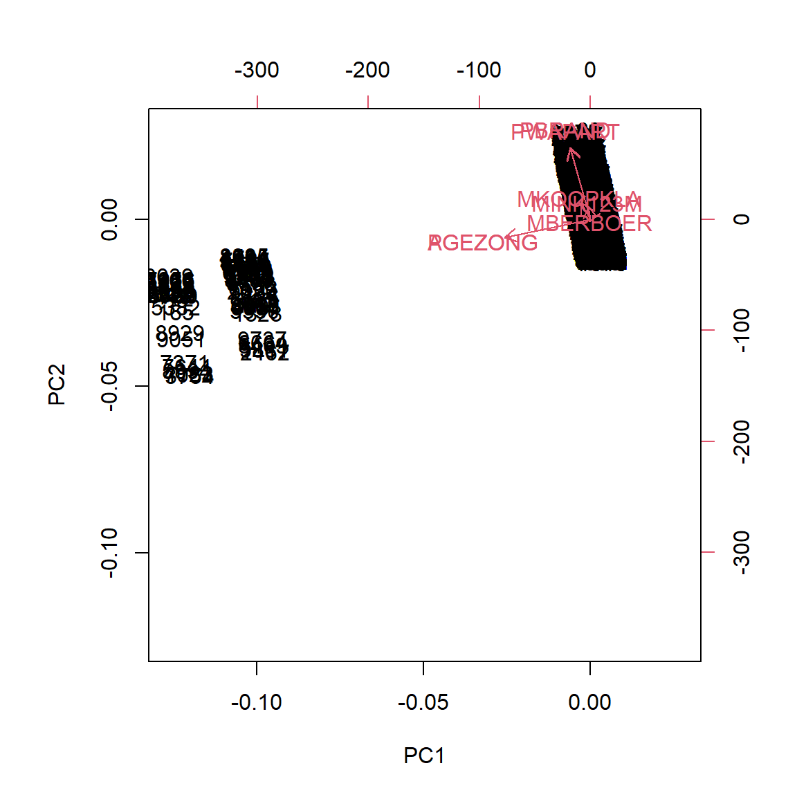
Even reducing the feature set down to just 15 variables didn’t help clear up the component plot all that much. Let’s step up to a more advanced method of plotting to see if we can coherse some information out of this analysis.
fviz_pca_biplot(cic_sm.pca, geom="point",
          pointshape=21,
          fill.ind = as.factor(cic_data$CARAVAN),
          col.ind = as.factor(cic_data$CARAVAN),
          col.var = "black",
          legend.title="CARAVAN",
          palette = "jco",
          addEllipses = TRUE,
          repel = TRUE, title="PCA-2d plot, 15 feature set")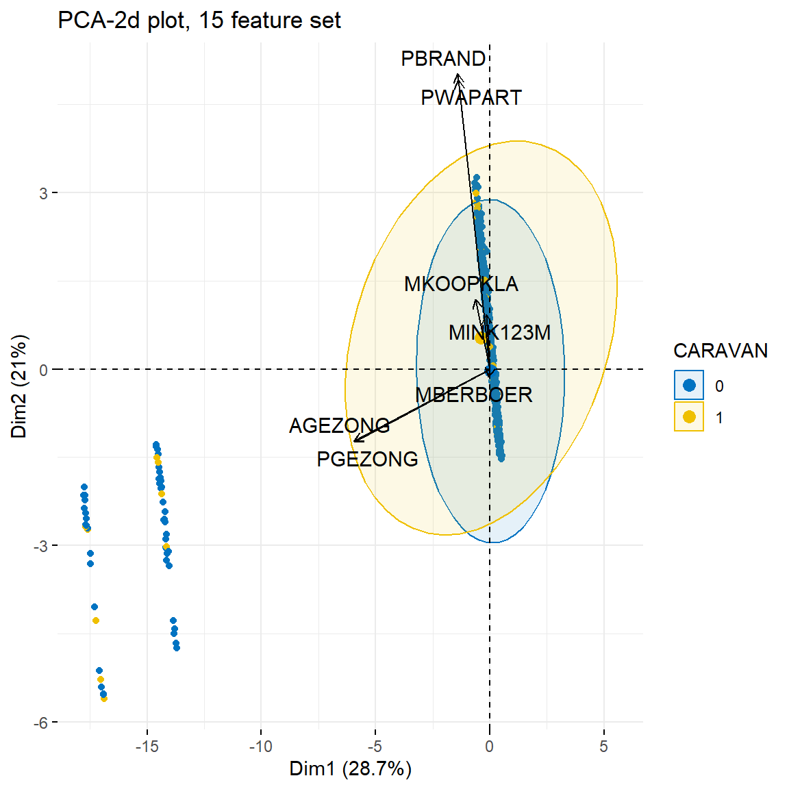
Using factoextra’s biplot certainly improves plot aesthetics but as
for uncovering additional useful information, that is debateable. We get
a better sense of the how disjoint the two groups are, but we would need
to dig deeper by experiementing with other features to realistically
understand if there is any insight to be gained here. At best, we can
say we have slightly stronger evidence supporting the idea that
A and P prefixes are just two ways of
representing the same value, but the correlation matrix in the previous notebook still supports that claim far better.
Recursive feature elimination
Recursive feature elimination is a greedy optimization algorithm that serves the same purpose as stepwise feature selection but does so in a different manner.
Rather than using a rigidly defined criteria metric such as p-value or AIC, RFE uses feature importance as determined by the model on which it is run. Both methods iterate through the model multiple times making modifications to the feature set, but RFE restores all features after each iteration, keeping track of how important each variable has been to the model in previous generations.
# Swap to random forest instead of linear model
ctrl <- rfeControl(method = "cv", number = 5, returnResamp = "all", functions = rfFuncs)

rfProfile <- rfe(subset(cic_data, select = -CARAVAN),
                 as.factor(cic_data$CARAVAN),
                 sizes=c(4,8,16,32,64,85),
                 rfeControl = ctrl)

rfProfile
##
## Recursive feature selection
##
## Outer resampling method: Cross-Validated (5 fold)
##
## Resampling performance over subset size:
##
## Variables Accuracy Kappa AccuracySD KappaSD Selected
## 4 0.9405 0.01225 0.0004134 0.01276 *
## 8 0.9402 0.01154 0.0007610 0.01258
## 16 0.9326 0.06899 0.0027723 0.01965
## 32 0.9331 0.08176 0.0034233 0.02369
## 64 0.9337 0.06494 0.0030347 0.01088
## 85 0.9340 0.05360 0.0030838 0.01741
##
## The top 4 variables (out of 4):
## PPERSAUT, PBRAND, APLEZIER, MOSTYPEplot(rfProfile, type = c("g", "o"))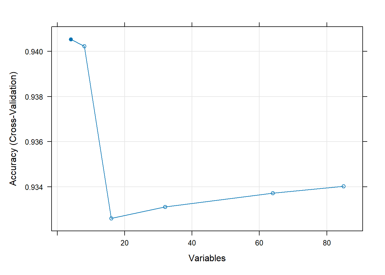
Interestingly, we can see here how additional variables actually
decrease the accuracy of the random forest model we are using. As
mentioned in the previous notebook’s analysis of this dataset, 94% is
the accuracy score a model would achieve by simply predicting all
FALSE values. So, to a certain degree, it is a good thing
that the accuracy decreased at first. Otherwise, if the accuracy stayed
at 94%, the model would not have even attempted to classify any
TRUE values at all.
plot1 <- xyplot(rfProfile,
                type = c("g", "p", "smooth"),
                ylab = "RMSE CV Estimates")
plot2 <- densityplot(rfProfile,
                     subset = Variables < 5,
                     adjust = 1.25,
                     as.table = TRUE,
                     xlab = "RMSE CV Estimates",
                     pch = "|")
print(plot1, split=c(1,1,1,2), more=TRUE)
print(plot2, split=c(1,2,1,2))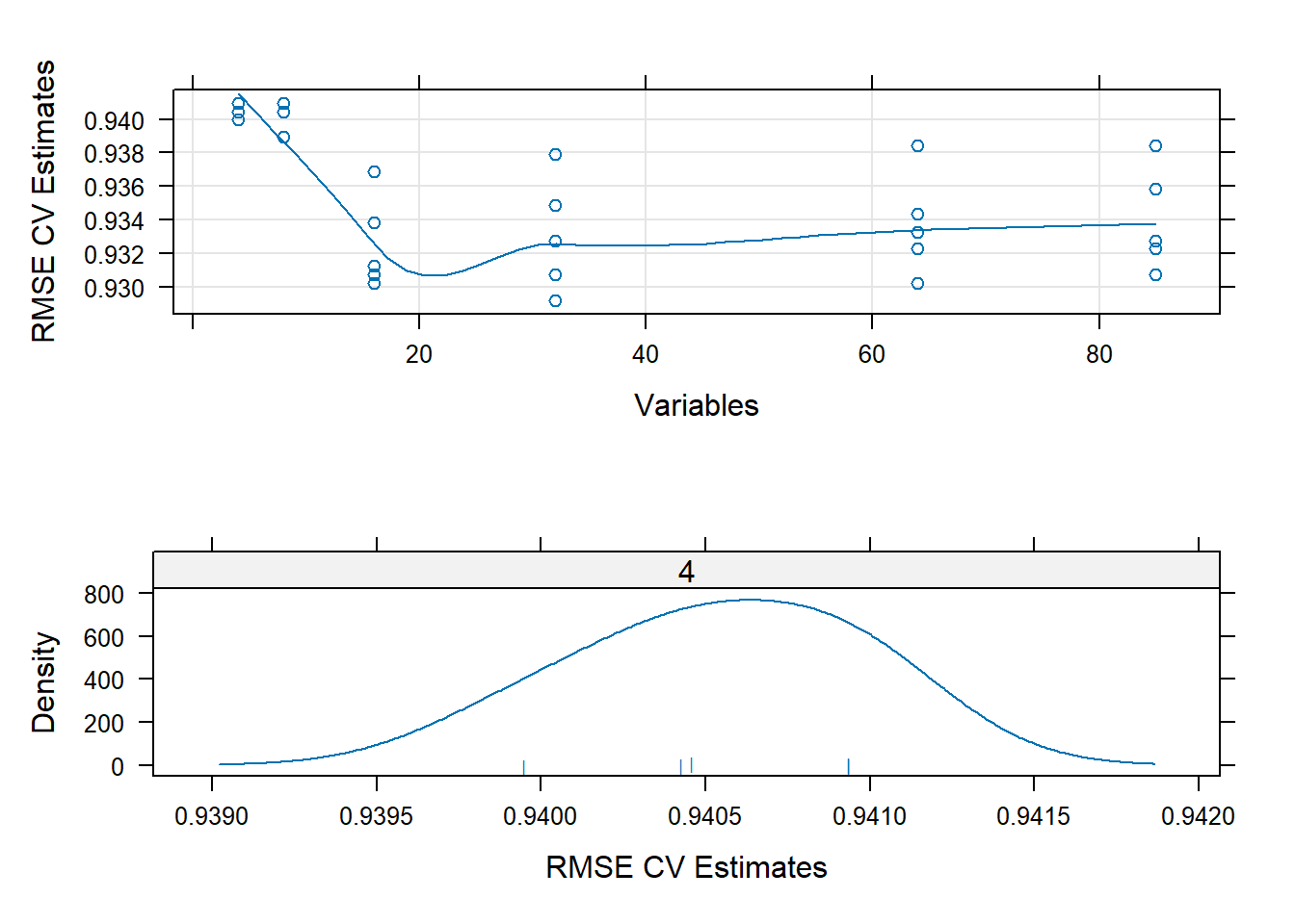
Again, here we can see how 0.940 is the central accurary score around which all others are distributed. With fewer variables, each fold of the cross validation is clustered closely around this score, but as new variables are introduced, they begin to spread across a slightly larger spectrum.
ctrl <- rfeControl(method = "cv", number = 5, returnResamp = "all", functions = rfFuncs)

ctrl$returnResamp <- "all"
rfProfile <- rfe(subset(cic_data, select = -CARAVAN),
                 as.factor(cic_data$CARAVAN),
                 sizes=c(4,8,16,32,64,85),
                 rfeControl = ctrl)
rfProfile
##
## Recursive feature selection
##
## Outer resampling method: Cross-Validated (5 fold)
##
## Resampling performance over subset size:
##
## Variables Accuracy Kappa AccuracySD KappaSD Selected
## 4 0.9403 0.008826 0.0009731 0.02143 *
## 8 0.9398 0.013427 0.0004208 0.01682
## 16 0.9305 0.056817 0.0013730 0.01397
## 32 0.9310 0.051068 0.0015589 0.02396
## 64 0.9331 0.046476 0.0025591 0.03512
## 85 0.9349 0.050660 0.0017526 0.02981
##
## The top 4 variables (out of 4):
## PPERSAUT, PBRAND, MOSTYPE, APLEZIERT-SNE
library(Rtsne)
# t-sne requires no duplicate values in the data, even if they are distinct and valid entries
cic_unq <- unique(subset(cic_data))
cic.tsne <- Rtsne(cic_unq,
theta=0.1, # precision where 0=exact t-sne, 1=fastest
num_threads = 4, # multicore
partial_pca = TRUE, # Fast PCA
pca_scale=TRUE,
initial_dims = 2,
perplexity=30,
verbose=TRUE,
max_iter = 1000)## Performing PCA
## Read the 8380 x 2 data matrix successfully!
## OpenMP is working. 4 threads.
## Using no_dims = 2, perplexity = 30.000000, and theta = 0.100000
## Computing input similarities...
## Building tree...
## Done in 0.29 seconds (sparsity = 0.012404)!
## Learning embedding...
## Iteration 50: error is 96.981510 (50 iterations in 2.21 seconds)
## Iteration 100: error is 78.790863 (50 iterations in 2.26 seconds)
## Iteration 150: error is 72.329301 (50 iterations in 1.82 seconds)
## Iteration 200: error is 69.006548 (50 iterations in 1.70 seconds)
## Iteration 250: error is 67.163294 (50 iterations in 1.83 seconds)
## Iteration 300: error is 2.232485 (50 iterations in 1.87 seconds)
## Iteration 350: error is 1.757471 (50 iterations in 1.83 seconds)
## Iteration 400: error is 1.477625 (50 iterations in 1.81 seconds)
## Iteration 450: error is 1.294077 (50 iterations in 1.80 seconds)
## Iteration 500: error is 1.165966 (50 iterations in 1.76 seconds)
## Iteration 550: error is 1.071931 (50 iterations in 1.76 seconds)
## Iteration 600: error is 1.000255 (50 iterations in 1.75 seconds)
## Iteration 650: error is 0.944040 (50 iterations in 1.74 seconds)
## Iteration 700: error is 0.898971 (50 iterations in 1.76 seconds)
## Iteration 750: error is 0.862316 (50 iterations in 1.71 seconds)
## Iteration 800: error is 0.831997 (50 iterations in 1.72 seconds)
## Iteration 850: error is 0.806537 (50 iterations in 1.69 seconds)
## Iteration 900: error is 0.784908 (50 iterations in 1.69 seconds)
## Iteration 950: error is 0.766340 (50 iterations in 1.69 seconds)
## Iteration 1000: error is 0.750230 (50 iterations in 1.69 seconds)
## Fitting performed in 36.10 seconds.cic.tsne$Y %>%
as.data.frame() %>%
ggplot(aes(x=V1, y=V2, color=as.factor(cic_unq$CARAVAN))) +
geom_point() +
scale_color_manual(values=c("gray", "red2")) +
labs(title="T-SNE 2-dims", color="CARAVAN")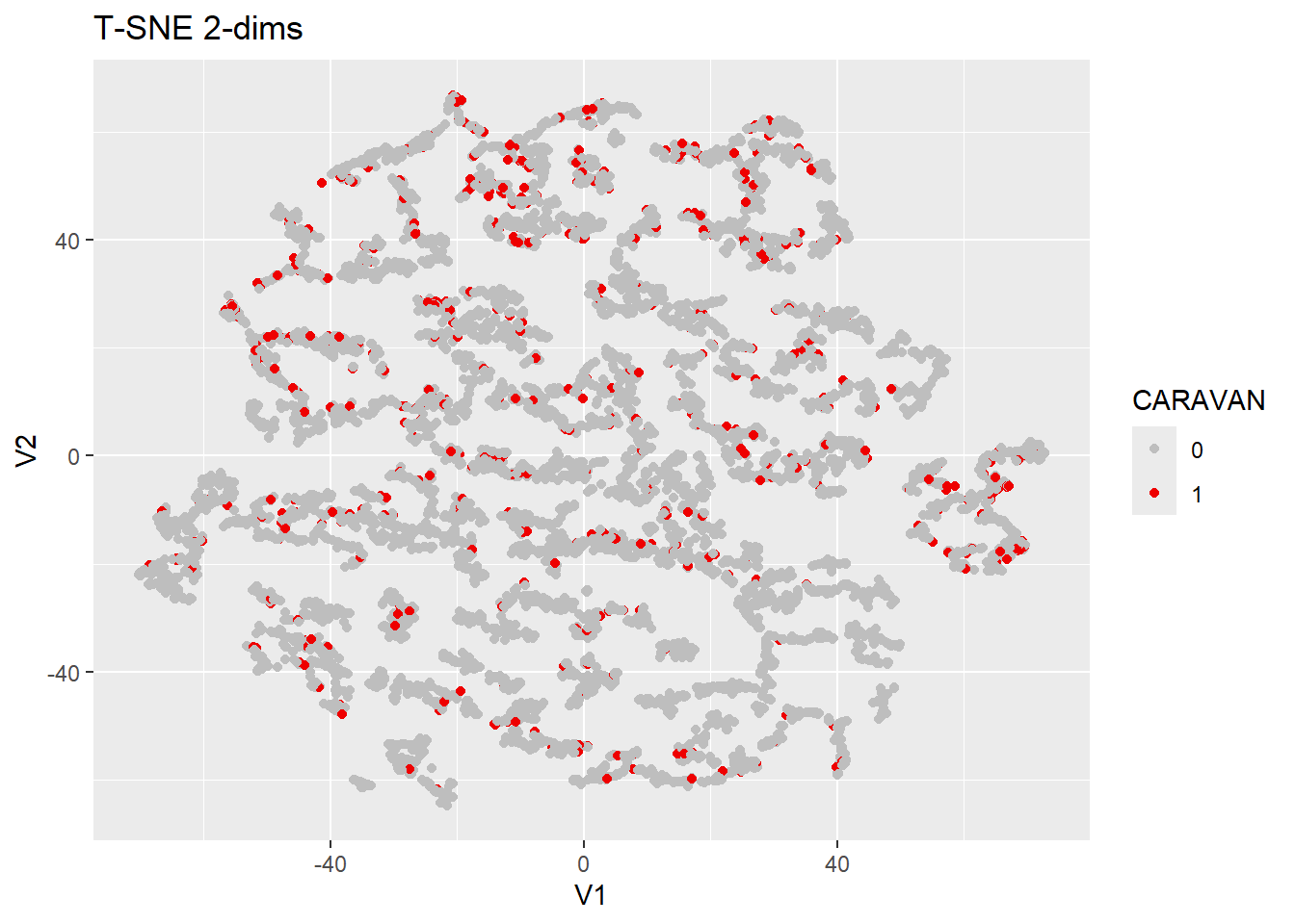
T-SNE does little to help delineate differences among the pos/neg
samples. There are many small clusters, but each contains both 0 and 1
response outcomes. That said, one advantage tsne offers is a high degree
of tweakability, adjustments to initial_dims or
perplexity could yield more interesting results, but
nothing immediately jumps out saying there is reason to explore these
options in great depth.
UMAP
library(umap)This R implementation of UMAP has some quirks about it, the easiest fix is just to make our own little wrapper around the function to get a better feel for what is going on.
# Extremely thin wrapper to be able to see all the possiable config params at a glance
umap.wrap <-
  function(d, # matrix; input data
           n_neighbors = 15, # integer; number of nearest neighbors
           n_components = 2, # integer; dimension of target (output) space
           metric = "euclidean", # see below
           n_epochs = 200, # integer; number of iterations performed during layout optimization
           input = "data", # c("data", "dist"); determines whether `d` is treated as a data matrix or a distance matrix
           init = "spectral", # see below
           min_dist = 0.1, #  determines how close points appear in the final layout
           set_op_mix_ratio = 1, # range [0,1]; determines who the knn-graph is used to create a fuzzy simplicial graph
           local_connectivity = 1, # used during construction of fuzzy simplicial set
           bandwidth = 1, # used during construction of fuzzy simplicial set
           alpha = 1, # initial value of "learning rate" of layout optimization
           gamma = 1, # determines, together with alpha, the learning rate of layout optimization
           negative_sample_rate = 5, # determines how many non-neighbor points used per point/iteration during layout optimization
           a = NA, # contributes to gradient calculations during layout optimization. Auto calcs when = NA
           b = NA, # contributes to gradient calculations during layout optimization
           spread = 1, # used during automatic estimation of a/b parameters.
           random_state = NA, # seed for random number generation used during umap()
           transform_state = NA, # seed for random number generation used during predict()
           knn=NA, # object of class umap.knn; precomputed nearest neighbors
           knn_repeats = 1, # number of times to restart knn search
           verbose = FALSE, # determines whether to show progress messages
           umap_learn_args = NA, # vector of arguments to python package umap-learn
           method= c("naive", "umap-learn")) # see below
  {
  params <- as.list(environment())
  conf <- params[2:(length(params)-1)]
  class(conf) <- "umap.config"

  return(umap(d=d, config=conf, method=method))
}metric: character or function; determines how distances between data points are computed. When using a string, available metrics are: c(“euclidean”, “manhattan”). Other available generalized metrics are: c(“cosine”, “pearson”, “pearson2”). Note: the triangle inequality may not be satisfied by some generalized metrics, hence knn search may not be optimal. When usingmetric.functionas a function, the signature must befunction(matrix, origin, target)and should compute a distance between the origin column and the target columnsinit: character or matrix; The default string “spectral” computes an initial embedding using eigenvectors of the connectivity graph matrix. An alternative is the string “random”, which creates an initial layout based on random coordinates. This setting.can also be set to a matrix, in which case layout optimization begins from the provided coordinates.method: character; implementation. Available methods are ‘naive’ (an implementation written in pure R) and ‘umap-learn’ (requires python package ‘umap-learn’)
Taken directly from https://cran.r-project.org/web/packages/umap/umap.pdf with slight stylistic modifications
cic.umap <- umap.wrap(subset(cic_data, select = -CARAVAN), n_epochs = 750, alpha=500, min_dist=.2)cic.umap$layout %>%
as.data.frame() %>%
ggplot(aes(V1, V2)) +
geom_point(aes(color=as.factor(cic_data$CARAVAN)))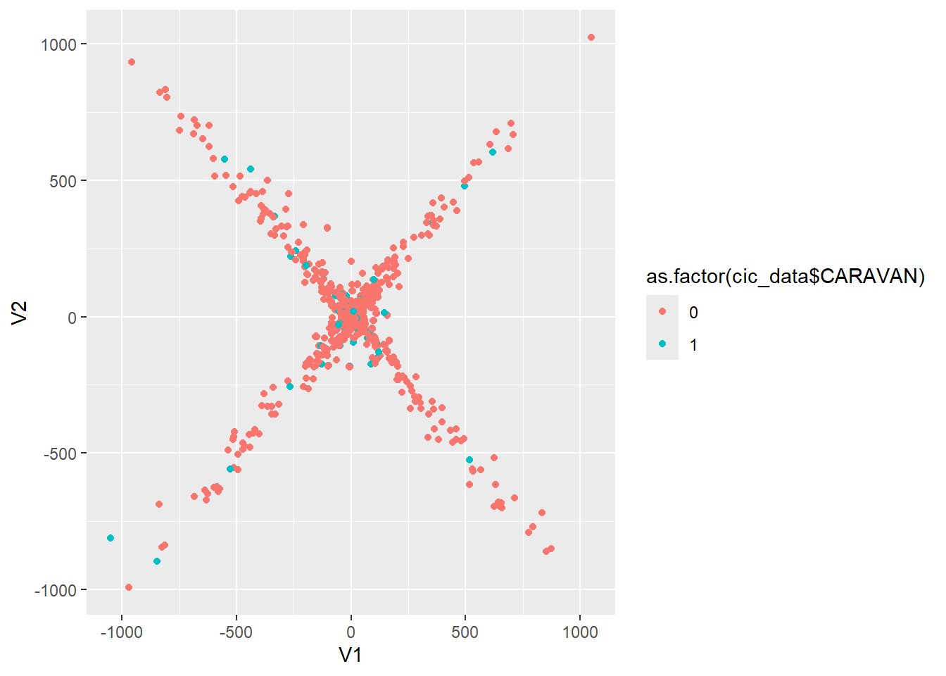
Our initial experimentation with UMAP does not indicate any clearly distinguishable difference between the classes. Perhaps with a bit of parameter tweaking we can coerce useful information out of this algorithm.
cic.umap.lt <- umap.wrap(d=subset(cic_data, select = -CARAVAN), n_neighbors = 10, n_epochs=350, verbose = TRUE)cic.umap.lt$layout %>% as.data.frame() %>%
ggplot(aes(V1, V2)) +
geom_point(aes(color=as.factor(cic_data$CARAVAN)))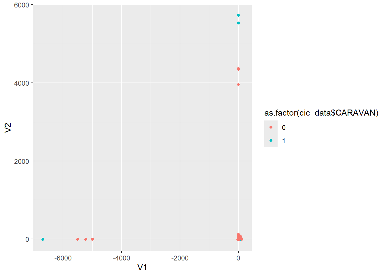
An interesting pattern, to say the least, but we can see by the large intermixed cluster at 0,0 UMAP also is not yielding ideal results in terms of interpretability.
# TODO : Feature importance random forest
# rfFuncs$rank()
Conclusions
This notebook was a complement to, or extension of, the previous previous notebook looking at the CoIL 2000 dataset. The focus this time was more on finding interesting features rather than trying many models. We used p-values from Ordinary Least Squares to perform step-wise feature selection and found 16 statistically significant features.
Thereafter, we performed PCA on both a non-standardized and standardized dataset and plotted scatter and density for each. Following that, we used two non-linear dimensionality reduction techniques, t-SNE and UMAP and looked at how those fared with the data.
We closeout with by taking a look at feature importance with a Random Forest model and performing Recursive Feature Elimination on both that and a Logistic Regressor. We find that the two models share a handful of features in common after elimination, both finding 42 variables worth keeping but only 14 of which were common between them.
The sweet spot for features seems to be between 42 and 64, as this range can explain over 90% of variance and houses 90% of importance in our Random Forest model.
Future work:
There are quite a few other dimensionality reduction techniques that could be tried, ISOMAP, SOM, Sammson mapping, and many more, all of which could provide more insight into the data. The question still remains as to whether or not the presumed redundant variables can be removed without negatively impacting predictive power. This should be explored in great depth now that we have more evidence supporting the claim. Additionally, it would be interesting to see if some form of semi-supervised learning approach could be used via k-means clustering or a similar approach.