Multiple Linear Regression
Overview
This document will fit a multiple linear model on two separate datasets: Boston from the MASS library, and Carseats from the ISLR library.
Various methods will be used to better the models created including:
- Removal of insignificant predictors
- Removal of highly collinear predictors
- Addition of polynomial terms
- Addition of interaction terms
Imports
library(MASS)
library(ISLR)
library(car)
#library(ggplot2)
library(tidyverse)
library(magrittr)
Boston
Data
This dataset is from the MASS library, it contains information collected by the U.S Census Service in 1970 concerning housing in the area of Boston Mass.
The dataset contains 506 and 14 columns:
crim- per capita crime rate by town.zn- proportion of residential land zoned for lots over 25,000 sq.ft.indus- proportion of non-retail business acres per town.chas- Charles River dummy variable (= 1 if tract bounds river; 0 otherwise).nox- nitrogen oxides concentration (parts per 10 million).rm- average number of rooms per dwelling.age- proportion of owner-occupied units built prior to 1940.dis- weighted mean of distances to five Boston employment centres.rad- index of accessibility to radial highways.tax- full-value property-tax rate per $10,000.ptratio- pupil-teacher ratio by town.black- 1000(Bk - 0.63)^2 where Bk is the proportion of blacks by town.lstat- lower status of the population (percent).medv- median value of owner-occupied homes in $1000s.
Additional information can be found:
https://stat.ethz.ch/R-manual/R-devel/library/MASS/html/Boston.html
https://www.cs.toronto.edu/~delve/data/boston/bostonDetail.html
http://citeseerx.ist.psu.edu/viewdoc/download?doi=10.1.1.926.5532&rep=rep1&type=pdf
or by typing ?Boston after importing MASS
head(bm <- MASS::Boston, n=10)Exploratory Data Analysis
The Boston dataset has no missing values and contains only numeric data, though this far from an extensive data assessment, for the purposes of this demonstration, the data can be assumed clean enough. A more thorough assessment could be performed by reading the original paper to see if the author filled in any missing values or specified any other manipulations.
all(complete.cases(bm))## [1] TRUEstr(bm)## 'data.frame': 506 obs. of 14 variables:
## $ crim : num 0.00632 0.02731 0.02729 0.03237 0.06905 ...
## $ zn : num 18 0 0 0 0 0 12.5 12.5 12.5 12.5 ...
## $ indus : num 2.31 7.07 7.07 2.18 2.18 2.18 7.87 7.87 7.87 7.87 ...
## $ chas : int 0 0 0 0 0 0 0 0 0 0 ...
## $ nox : num 0.538 0.469 0.469 0.458 0.458 0.458 0.524 0.524 0.524 0.524 ...
## $ rm : num 6.58 6.42 7.18 7 7.15 ...
## $ age : num 65.2 78.9 61.1 45.8 54.2 58.7 66.6 96.1 100 85.9 ...
## $ dis : num 4.09 4.97 4.97 6.06 6.06 ...
## $ rad : int 1 2 2 3 3 3 5 5 5 5 ...
## $ tax : num 296 242 242 222 222 222 311 311 311 311 ...
## $ ptratio: num 15.3 17.8 17.8 18.7 18.7 18.7 15.2 15.2 15.2 15.2 ...
## $ black : num 397 397 393 395 397 ...
## $ lstat : num 4.98 9.14 4.03 2.94 5.33 ...
## $ medv : num 24 21.6 34.7 33.4 36.2 28.7 22.9 27.1 16.5 18.9 ...plot(bm)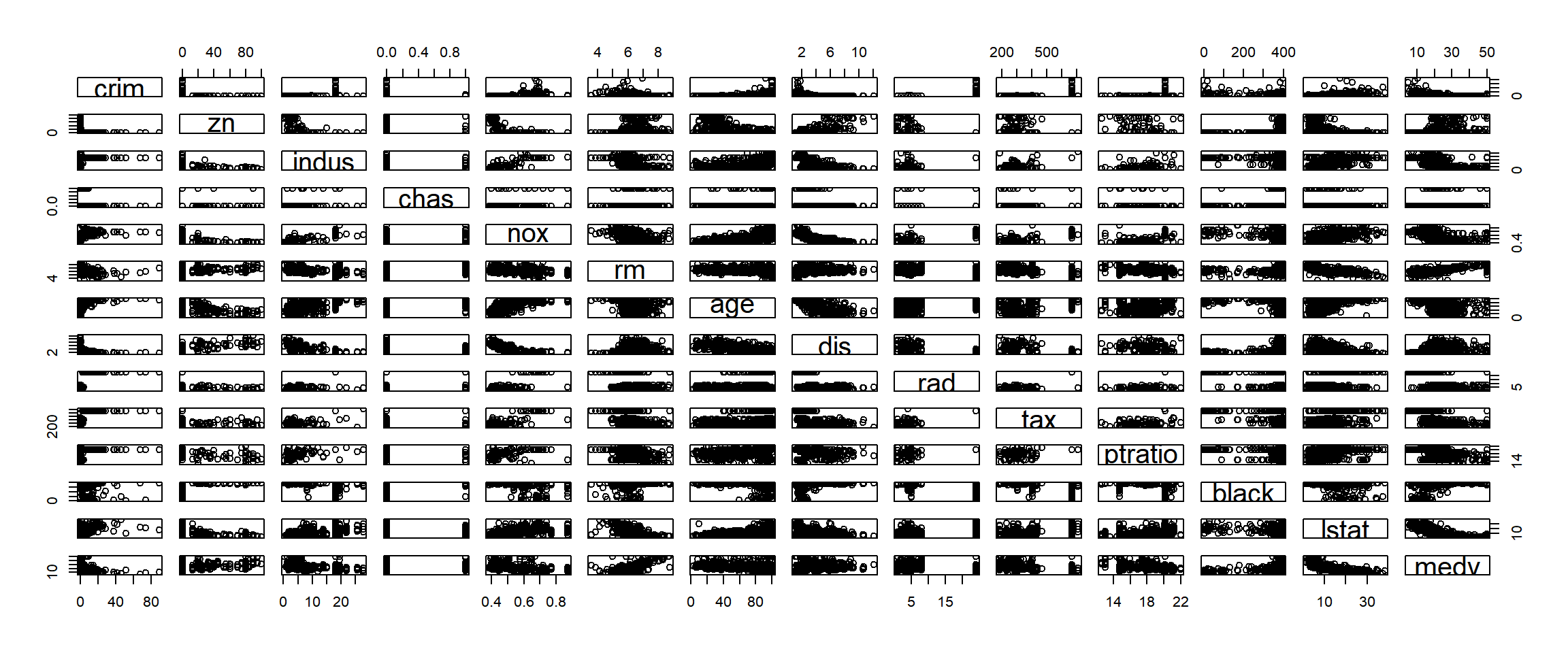 From a quick plot, we can see a quite a few possible linear relationship candidates: rm:zn, dis:zn, nox:dis, nox:age, rm:lstat, …
Looking exclusively at medv relationships:
medv:lstat, medv:rm, medv:age, medv:zn
par(mfrow=c(2,2))
plot(medv~lstat + rm + age + zn, data=bm)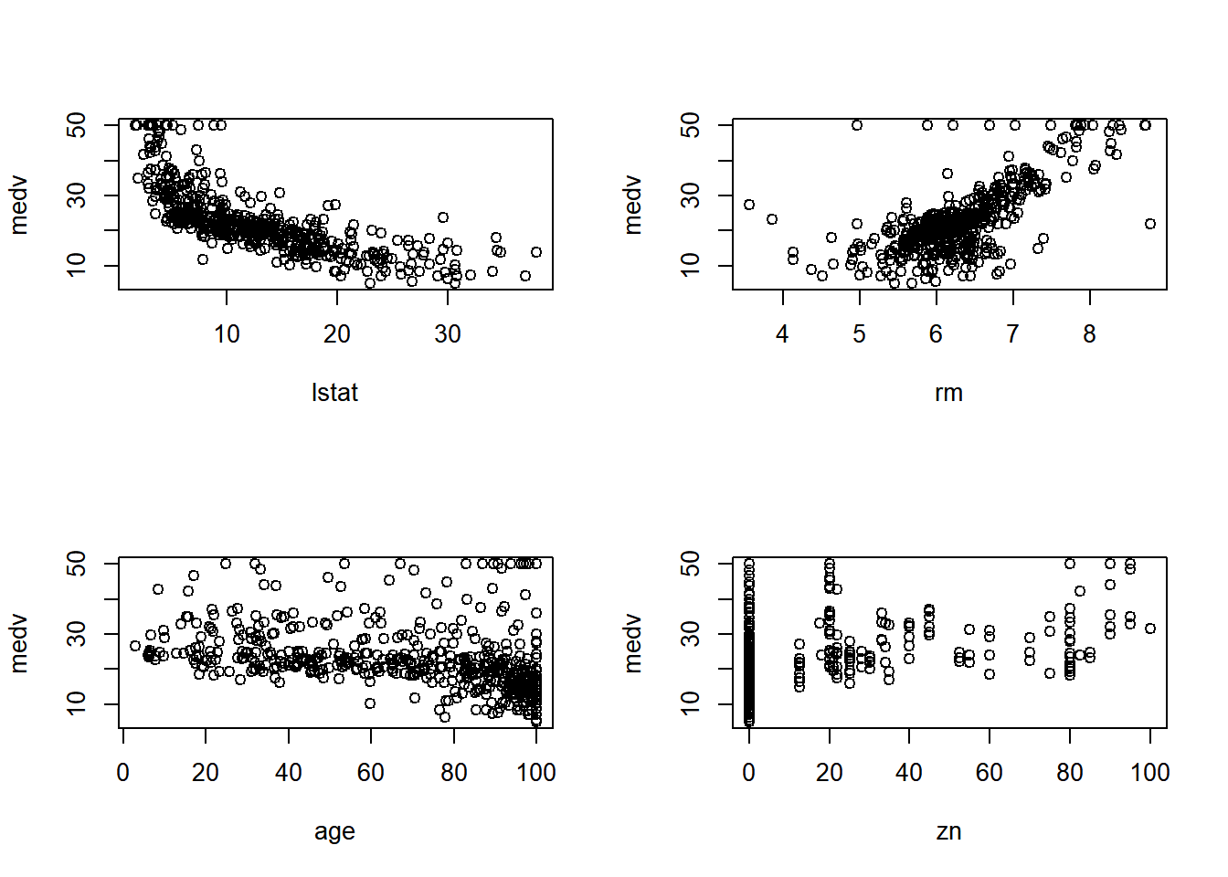
summary(lm(bm$medv ~ . ,data=bm))##
## Call:
## lm(formula = bm$medv ~ ., data = bm)
##
## Residuals:
## Min 1Q Median 3Q Max
## -15.595 -2.730 -0.518 1.777 26.199
##
## Coefficients:
## Estimate Std. Error t value Pr(>|t|)
## (Intercept) 3.646e+01 5.103e+00 7.144 3.28e-12 ***
## crim -1.080e-01 3.286e-02 -3.287 0.001087 **
## zn 4.642e-02 1.373e-02 3.382 0.000778 ***
## indus 2.056e-02 6.150e-02 0.334 0.738288
## chas 2.687e+00 8.616e-01 3.118 0.001925 **
## nox -1.777e+01 3.820e+00 -4.651 4.25e-06 ***
## rm 3.810e+00 4.179e-01 9.116 < 2e-16 ***
## age 6.922e-04 1.321e-02 0.052 0.958229
## dis -1.476e+00 1.995e-01 -7.398 6.01e-13 ***
## rad 3.060e-01 6.635e-02 4.613 5.07e-06 ***
## tax -1.233e-02 3.760e-03 -3.280 0.001112 **
## ptratio -9.527e-01 1.308e-01 -7.283 1.31e-12 ***
## black 9.312e-03 2.686e-03 3.467 0.000573 ***
## lstat -5.248e-01 5.072e-02 -10.347 < 2e-16 ***
## ---
## Signif. codes: 0 '***' 0.001 '**' 0.01 '*' 0.05 '.' 0.1 ' ' 1
##
## Residual standard error: 4.745 on 492 degrees of freedom
## Multiple R-squared: 0.7406, Adjusted R-squared: 0.7338
## F-statistic: 108.1 on 13 and 492 DF, p-value: < 2.2e-16Taking a more scientifically rigorous approach, we can see why simply looking at plots can be misleading.
lstat and rm are extremely good, with a p-value even smaller than machine epsilon, zn meets the p=0.05 threshold, but age turns out to be well beyond any useful significance level.
Additionally, there were several variables whose plots did not immediately show obvious correlation that also have extremely low p-values:
        t-value  p-value
dis      -7.398  6.01e-13 ***
ptratio  -7.283  1.31e-12 ***
par(mfrow=c(1,2))
plot(medv ~ dis + ptratio, data=bm)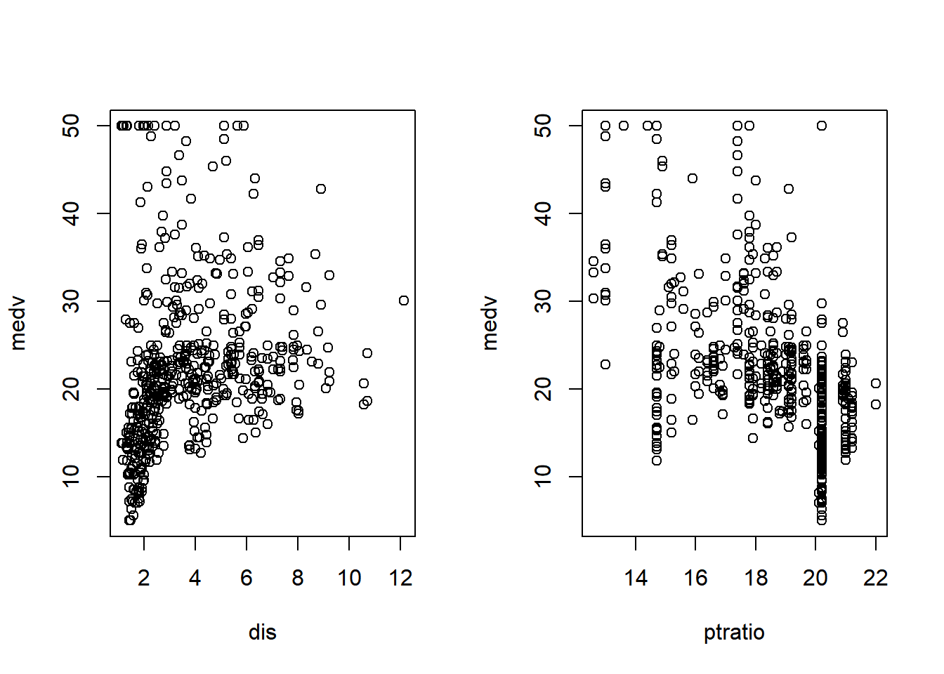
Check the data for correlations with Variance Inflation Factors
vif(lm(medv ~ ., data=bm))## crim zn indus chas nox rm age dis
## 1.792192 2.298758 3.991596 1.073995 4.393720 1.933744 3.100826 3.955945
## rad tax ptratio black lstat
## 7.484496 9.008554 1.799084 1.348521 2.941491vif(lm(medv ~ rad+tax, data=bm))## rad tax
## 5.831426 5.831426There are some highly correlated values among predictors, before we are able to make a suitable model, this issue will need to be addressed. As a general rule of thumb, VIF of > 5 means that the variable should be looked at to determine if there are issues, VIF > 10, that variable is almost certainly causing colinearity issues.
AIC(lm(medv ~ . ,data=bm))## [1] 3027.609BIC(lm(medv ~ . ,data=bm))## [1] 3091.007Models
The baseline values for our multiple linear model are:
Multiple R-squared: 0.7406, Adjusted R-squared: 0.7338, AIC: 3027.609, BIC: 3091.007
After a bit of feature selection and added polynomial terms the final model values are: Multiple R-squared: 0.8168, Adjusted R-squared: 0.8120, AIC: 2851.624, BIC: 2915.022
A fairly sizable improvement across the board
# exclude variables where p>0.05
summary(lm(medv ~. - age - indus, data=bm))
##
## Call:
## lm(formula = medv ~ . - age - indus, data = bm)
##
## Residuals:
## Min 1Q Median 3Q Max
## -15.5984 -2.7386 -0.5046 1.7273 26.2373
##
## Coefficients:
## Estimate Std. Error t value Pr(>|t|)
## (Intercept) 36.341145 5.067492 7.171 2.73e-12 ***
## crim -0.108413 0.032779 -3.307 0.001010 **
## zn 0.045845 0.013523 3.390 0.000754 ***
## chas 2.718716 0.854240 3.183 0.001551 **
## nox -17.376023 3.535243 -4.915 1.21e-06 ***
## rm 3.801579 0.406316 9.356 < 2e-16 ***
## dis -1.492711 0.185731 -8.037 6.84e-15 ***
## rad 0.299608 0.063402 4.726 3.00e-06 ***
## tax -0.011778 0.003372 -3.493 0.000521 ***
## ptratio -0.946525 0.129066 -7.334 9.24e-13 ***
## black 0.009291 0.002674 3.475 0.000557 ***
## lstat -0.522553 0.047424 -11.019 < 2e-16 ***
## ---
## Signif. codes: 0 '***' 0.001 '**' 0.01 '*' 0.05 '.' 0.1 ' ' 1
##
## Residual standard error: 4.736 on 494 degrees of freedom
## Multiple R-squared: 0.7406, Adjusted R-squared: 0.7348
## F-statistic: 128.2 on 11 and 494 DF, p-value: < 2.2e-16Excluding age and indus from the model slightly improves the adjusted R-squared value.
smry <- summary(lm(medv~. ,data=bm))
smry$coefficients
## Estimate Std. Error t value Pr(>|t|)
## (Intercept) 3.645949e+01 5.103458811 7.14407419 3.283438e-12
## crim -1.080114e-01 0.032864994 -3.28651687 1.086810e-03
## zn 4.642046e-02 0.013727462 3.38157628 7.781097e-04
## indus 2.055863e-02 0.061495689 0.33431004 7.382881e-01
## chas 2.686734e+00 0.861579756 3.11838086 1.925030e-03
## nox -1.776661e+01 3.819743707 -4.65125741 4.245644e-06
## rm 3.809865e+00 0.417925254 9.11614020 1.979441e-18
## age 6.922246e-04 0.013209782 0.05240243 9.582293e-01
## dis -1.475567e+00 0.199454735 -7.39800360 6.013491e-13
## rad 3.060495e-01 0.066346440 4.61289977 5.070529e-06
## tax -1.233459e-02 0.003760536 -3.28000914 1.111637e-03
## ptratio -9.527472e-01 0.130826756 -7.28251056 1.308835e-12
## black 9.311683e-03 0.002685965 3.46679256 5.728592e-04
## lstat -5.247584e-01 0.050715278 -10.34714580 7.776912e-23summary(lm(medv~. ,data=bm))##
## Call:
## lm(formula = medv ~ ., data = bm)
##
## Residuals:
## Min 1Q Median 3Q Max
## -15.595 -2.730 -0.518 1.777 26.199
##
## Coefficients:
## Estimate Std. Error t value Pr(>|t|)
## (Intercept) 3.646e+01 5.103e+00 7.144 3.28e-12 ***
## crim -1.080e-01 3.286e-02 -3.287 0.001087 **
## zn 4.642e-02 1.373e-02 3.382 0.000778 ***
## indus 2.056e-02 6.150e-02 0.334 0.738288
## chas 2.687e+00 8.616e-01 3.118 0.001925 **
## nox -1.777e+01 3.820e+00 -4.651 4.25e-06 ***
## rm 3.810e+00 4.179e-01 9.116 < 2e-16 ***
## age 6.922e-04 1.321e-02 0.052 0.958229
## dis -1.476e+00 1.995e-01 -7.398 6.01e-13 ***
## rad 3.060e-01 6.635e-02 4.613 5.07e-06 ***
## tax -1.233e-02 3.760e-03 -3.280 0.001112 **
## ptratio -9.527e-01 1.308e-01 -7.283 1.31e-12 ***
## black 9.312e-03 2.686e-03 3.467 0.000573 ***
## lstat -5.248e-01 5.072e-02 -10.347 < 2e-16 ***
## ---
## Signif. codes: 0 '***' 0.001 '**' 0.01 '*' 0.05 '.' 0.1 ' ' 1
##
## Residual standard error: 4.745 on 492 degrees of freedom
## Multiple R-squared: 0.7406, Adjusted R-squared: 0.7338
## F-statistic: 108.1 on 13 and 492 DF, p-value: < 2.2e-16head(bm[smry$coefficients[,4] < 5e-4],20)summary(lm(medv ~. -age -indus -crim -chas -zn -tax -rad -black, data=bm))##
## Call:
## lm(formula = medv ~ . - age - indus - crim - chas - zn - tax -
## rad - black, data = bm)
##
## Residuals:
## Min 1Q Median 3Q Max
## -12.7765 -3.0186 -0.6481 1.9752 27.7625
##
## Coefficients:
## Estimate Std. Error t value Pr(>|t|)
## (Intercept) 37.49920 4.61295 8.129 3.43e-15 ***
## nox -17.99657 3.26095 -5.519 5.49e-08 ***
## rm 4.16331 0.41203 10.104 < 2e-16 ***
## dis -1.18466 0.16842 -7.034 6.64e-12 ***
## ptratio -1.04577 0.11352 -9.212 < 2e-16 ***
## lstat -0.58108 0.04794 -12.122 < 2e-16 ***
## ---
## Signif. codes: 0 '***' 0.001 '**' 0.01 '*' 0.05 '.' 0.1 ' ' 1
##
## Residual standard error: 4.994 on 500 degrees of freedom
## Multiple R-squared: 0.7081, Adjusted R-squared: 0.7052
## F-statistic: 242.6 on 5 and 500 DF, p-value: < 2.2e-16# summary(lm(medv ~ nox +rm +dis +ptratio +lstat, data=bm)) # equivalentlyDropping all but the strongest indicators has reduced the R? value from 0.7348 to 0.7052 but has greatly simplified the model. Depending on the use case this may or may not be desirable, for the purposes of this demonstration, the simpler model will suffice.
vif(lm(bm$medv ~ lstat +rm +ptratio +dis +nox, data=bm))## lstat rm ptratio dis nox
## 2.373021 1.697104 1.223051 2.546968 2.891388vif(lm(medv ~ dis +nox, data=bm))## dis nox
## 2.449269 2.449269By reducing the number of parameters, much of the issues with collinearity among predictors has been resolved. A moderate correlation still exists in dis and nox, but not likely strong enough to cause large distortions in the model.
# build a model from the five lowest p-values
lm_lrpdn <- lm(medv ~ lstat +rm +ptratio +dis +nox, data=bm)
summary(lm_lrpdn)
##
## Call:
## lm(formula = medv ~ lstat + rm + ptratio + dis + nox, data = bm)
##
## Residuals:
## Min 1Q Median 3Q Max
## -12.7765 -3.0186 -0.6481 1.9752 27.7625
##
## Coefficients:
## Estimate Std. Error t value Pr(>|t|)
## (Intercept) 37.49920 4.61295 8.129 3.43e-15 ***
## lstat -0.58108 0.04794 -12.122 < 2e-16 ***
## rm 4.16331 0.41203 10.104 < 2e-16 ***
## ptratio -1.04577 0.11352 -9.212 < 2e-16 ***
## dis -1.18466 0.16842 -7.034 6.64e-12 ***
## nox -17.99657 3.26095 -5.519 5.49e-08 ***
## ---
## Signif. codes: 0 '***' 0.001 '**' 0.01 '*' 0.05 '.' 0.1 ' ' 1
##
## Residual standard error: 4.994 on 500 degrees of freedom
## Multiple R-squared: 0.7081, Adjusted R-squared: 0.7052
## F-statistic: 242.6 on 5 and 500 DF, p-value: < 2.2e-16lm_poly <- lm(medv ~ poly(lstat,5) +poly(rm,5) +ptratio +dis +nox, data=bm)
summary(lm_poly)##
## Call:
## lm(formula = medv ~ poly(lstat, 5) + poly(rm, 5) + ptratio +
## dis + nox, data = bm)
##
## Residuals:
## Min 1Q Median 3Q Max
## -12.4690 -2.0743 -0.2638 1.5585 27.8069
##
## Coefficients:
## Estimate Std. Error t value Pr(>|t|)
## (Intercept) 46.48539 2.77936 16.725 < 2e-16 ***
## poly(lstat, 5)1 -110.31734 6.72048 -16.415 < 2e-16 ***
## poly(lstat, 5)2 27.60368 5.37979 5.131 4.15e-07 ***
## poly(lstat, 5)3 -5.04740 4.46669 -1.130 0.259022
## poly(lstat, 5)4 12.78329 4.17450 3.062 0.002317 **
## poly(lstat, 5)5 -10.93446 4.22013 -2.591 0.009853 **
## poly(rm, 5)1 55.28702 5.85973 9.435 < 2e-16 ***
## poly(rm, 5)2 42.95462 4.85297 8.851 < 2e-16 ***
## poly(rm, 5)3 -0.50354 4.27075 -0.118 0.906191
## poly(rm, 5)4 -19.46204 4.58248 -4.247 2.59e-05 ***
## poly(rm, 5)5 -15.27024 4.41022 -3.462 0.000582 ***
## ptratio -0.67257 0.09579 -7.021 7.34e-12 ***
## dis -0.91151 0.13711 -6.648 7.90e-11 ***
## nox -14.56799 2.67333 -5.449 8.00e-08 ***
## ---
## Signif. codes: 0 '***' 0.001 '**' 0.01 '*' 0.05 '.' 0.1 ' ' 1
##
## Residual standard error: 3.988 on 492 degrees of freedom
## Multiple R-squared: 0.8168, Adjusted R-squared: 0.812
## F-statistic: 168.8 on 13 and 492 DF, p-value: < 2.2e-16From only two polynomial transforms we’ve improved the R-squared value significantly, now at 0.812, well beyond the original R-squared value of 0.7348 while using far fewer input variables.
# Before adding polynomial
print(paste('AIC:',round(AIC(lm_lrpdn),3), "BIC:",round(BIC(lm_lrpdn),3)),quote=FALSE)
## [1] AIC: 3071.439 BIC: 3101.024# After adding polynomial
print(paste('AIC:',round(AIC(lm_poly),3), "BIC:",round(BIC(lm_poly),3)), quote=FALSE)## [1] AIC: 2851.624 BIC: 2915.022The poly model also saw a decrease in AIC and BIC values
Akaike’s information criterion (AIC) and Bayesian information criterion (BIC) can be used to estimate the ‘goodness’ of a statistical model, both addressing the trade-off between goodness of fit and complexity in slightly different ways.
http://r-statistics.co/Linear-Regression.html
par(mfrow=c(2,2))
plot(lm_poly)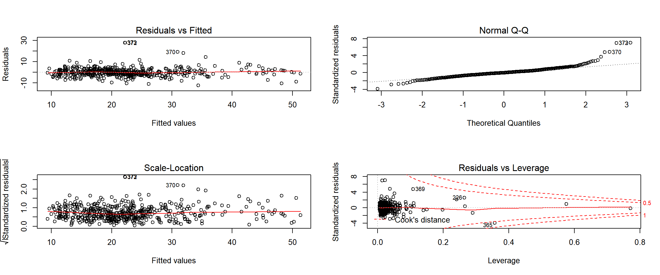
Carseats
Data
The data used in this notebook is from ISLR’s Carseats dataset. It represents simulated data of child carseat sales at 400 different stores with 11 variables:
Sales- Unit sales (in thousands) at each locationCompPrice- Price charged by competitor at each locationIncome- Community income level (in thousands of dollars)Advertising- Local advertising budget for company at each location (in thousands of dollars)Population- Population size in region (in thousands)Price- Price company charges for car seats at each siteShelveLoc- A factor with levels Bad, Good and Medium indicating the quality of the shelving location for the car seats at each siteAge- Average age of the local populationEducation- Education level at each locationUrban- A factor with levels No and Yes to indicate whether the store is in an urban or rural locationUS- A factor with levels No and Yes to indicate whether the store is in the US or not
Additional information can be found:
https://www.rdocumentation.org/packages/ISLR/versions/1.2/topics/Carseats
or by typing ?Carseats after importing ISLR
head(cs <- Carseats,n=20)Exploratory Data Analysis
Carseats is a simulated data set with no missing values. Being artificial, there is no reason to believe that the data is anything but clean. However, not all of the variables are numeric, so that is something worth keeping in mind when constructing models. There are 3 categorical variables, 2 binary (Urban,US) and 1 ordinal (ShelveLoc)
all(complete.cases(cs))## [1] TRUEstr(cs)## 'data.frame': 400 obs. of 11 variables:
## $ Sales : num 9.5 11.22 10.06 7.4 4.15 ...
## $ CompPrice : num 138 111 113 117 141 124 115 136 132 132 ...
## $ Income : num 73 48 35 100 64 113 105 81 110 113 ...
## $ Advertising: num 11 16 10 4 3 13 0 15 0 0 ...
## $ Population : num 276 260 269 466 340 501 45 425 108 131 ...
## $ Price : num 120 83 80 97 128 72 108 120 124 124 ...
## $ ShelveLoc : Factor w/ 3 levels "Bad","Good","Medium": 1 2 3 3 1 1 3 2 3 3 ...
## $ Age : num 42 65 59 55 38 78 71 67 76 76 ...
## $ Education : num 17 10 12 14 13 16 15 10 10 17 ...
## $ Urban : Factor w/ 2 levels "No","Yes": 2 2 2 2 2 1 2 2 1 1 ...
## $ US : Factor w/ 2 levels "No","Yes": 2 2 2 2 1 2 1 2 1 2 ...plot(cs)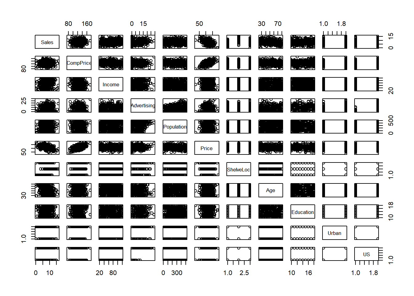
summary(lm(Sales ~ ., data=cs))##
## Call:
## lm(formula = Sales ~ ., data = cs)
##
## Residuals:
## Min 1Q Median 3Q Max
## -2.8692 -0.6908 0.0211 0.6636 3.4115
##
## Coefficients:
## Estimate Std. Error t value Pr(>|t|)
## (Intercept) 5.6606231 0.6034487 9.380 < 2e-16 ***
## CompPrice 0.0928153 0.0041477 22.378 < 2e-16 ***
## Income 0.0158028 0.0018451 8.565 2.58e-16 ***
## Advertising 0.1230951 0.0111237 11.066 < 2e-16 ***
## Population 0.0002079 0.0003705 0.561 0.575
## Price -0.0953579 0.0026711 -35.700 < 2e-16 ***
## ShelveLocGood 4.8501827 0.1531100 31.678 < 2e-16 ***
## ShelveLocMedium 1.9567148 0.1261056 15.516 < 2e-16 ***
## Age -0.0460452 0.0031817 -14.472 < 2e-16 ***
## Education -0.0211018 0.0197205 -1.070 0.285
## UrbanYes 0.1228864 0.1129761 1.088 0.277
## USYes -0.1840928 0.1498423 -1.229 0.220
## ---
## Signif. codes: 0 '***' 0.001 '**' 0.01 '*' 0.05 '.' 0.1 ' ' 1
##
## Residual standard error: 1.019 on 388 degrees of freedom
## Multiple R-squared: 0.8734, Adjusted R-squared: 0.8698
## F-statistic: 243.4 on 11 and 388 DF, p-value: < 2.2e-16R handles the dummy encoding of categorical variables for us so long as they are designated as factors rather than chars
summary(lm(cs$Sales ~. -Population -Education -Urban -US, data=cs))##
## Call:
## lm(formula = cs$Sales ~ . - Population - Education - Urban -
## US, data = cs)
##
## Residuals:
## Min 1Q Median 3Q Max
## -2.7728 -0.6954 0.0282 0.6732 3.3292
##
## Coefficients:
## Estimate Std. Error t value Pr(>|t|)
## (Intercept) 5.475226 0.505005 10.84 <2e-16 ***
## CompPrice 0.092571 0.004123 22.45 <2e-16 ***
## Income 0.015785 0.001838 8.59 <2e-16 ***
## Advertising 0.115903 0.007724 15.01 <2e-16 ***
## Price -0.095319 0.002670 -35.70 <2e-16 ***
## ShelveLocGood 4.835675 0.152499 31.71 <2e-16 ***
## ShelveLocMedium 1.951993 0.125375 15.57 <2e-16 ***
## Age -0.046128 0.003177 -14.52 <2e-16 ***
## ---
## Signif. codes: 0 '***' 0.001 '**' 0.01 '*' 0.05 '.' 0.1 ' ' 1
##
## Residual standard error: 1.019 on 392 degrees of freedom
## Multiple R-squared: 0.872, Adjusted R-squared: 0.8697
## F-statistic: 381.4 on 7 and 392 DF, p-value: < 2.2e-16Following a similar process as before, features outside of the statistical significance threshold are excluded.
This time, the adjusted R-squared value decreased but by so little, it could be safely written off as noise.
vif(lm(Sales ~., data=cs))## GVIF Df GVIF^(1/(2*Df))
## CompPrice 1.554618 1 1.246843
## Income 1.024731 1 1.012290
## Advertising 2.103136 1 1.450219
## Population 1.145534 1 1.070296
## Price 1.537068 1 1.239785
## ShelveLoc 1.033891 2 1.008367
## Age 1.021051 1 1.010471
## Education 1.026342 1 1.013086
## Urban 1.022705 1 1.011289
## US 1.980720 1 1.407380scs <- subset(cs, select=-c(Population, Education, Urban, US))
vif(lm(Sales ~., data=scs))## GVIF Df GVIF^(1/(2*Df))
## CompPrice 1.534883 1 1.238904
## Income 1.015448 1 1.007694
## Advertising 1.012935 1 1.006447
## Price 1.534425 1 1.238719
## ShelveLoc 1.015139 2 1.003763
## Age 1.016830 1 1.008380Neither the original nor the reduced data appear to have issues with high collinearity, so no further action is required before modeling
plot(scs)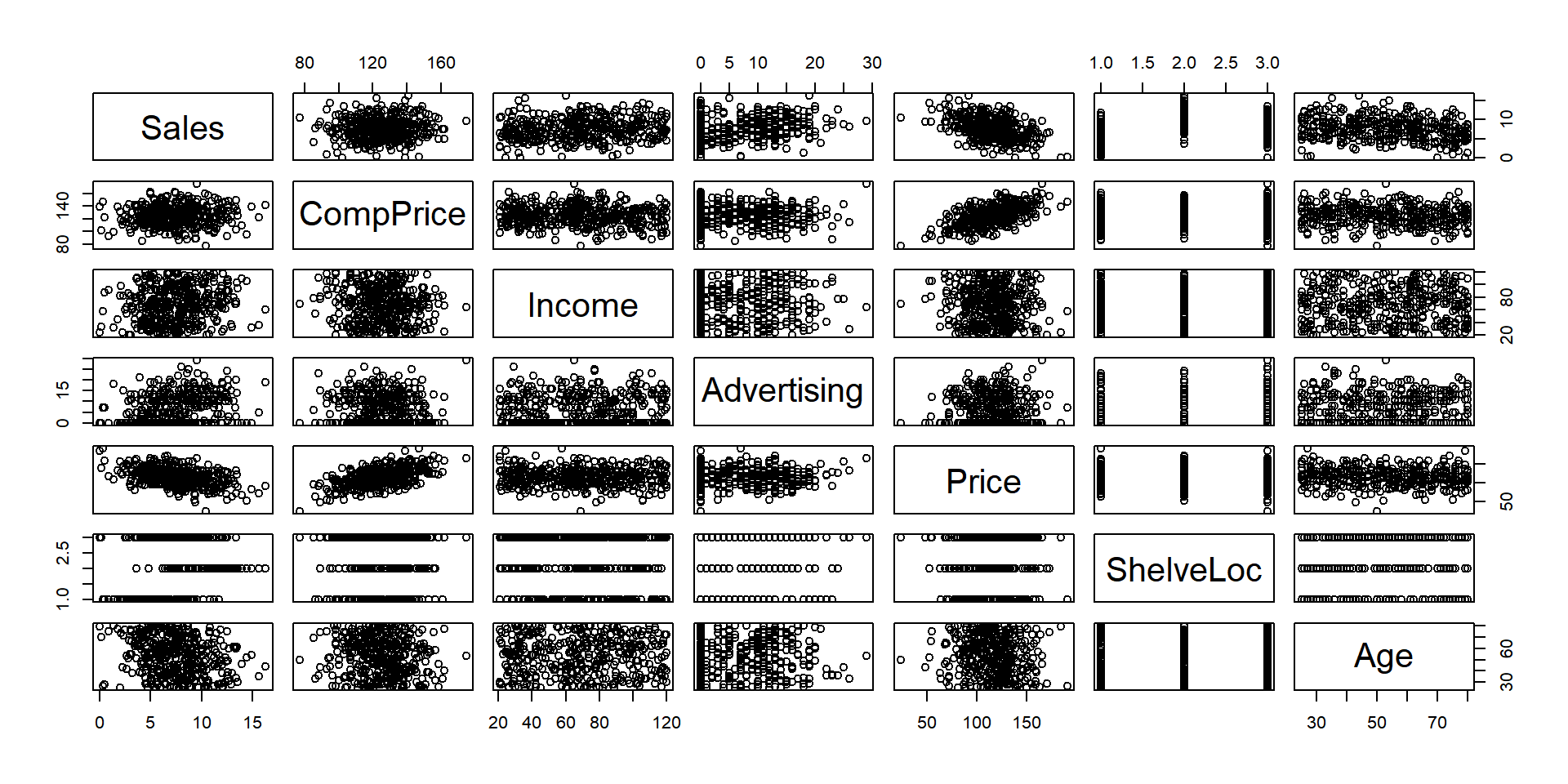
A quick plot shows potential for a linear relationships between Price and CompPrice/Sales
Models
The baseline values for our multiple linear model are:
Multiple R-squared: 0.8734, Adjusted R-squared: 0.8698, AIC: 1160.470, BIC: 1196.393
After feature selection, added polynomial and interaction terms, the final model values are:
Multiple R-squared: 0.8768, Adjusted R-squared: 0.8730, AIC: 1155.221, BIC: 1211.101
These results are far from ideal, only 3/4 metrics improved and only by a very small amount.
summary(lm(Sales ~ ., data=scs))##
## Call:
## lm(formula = Sales ~ ., data = scs)
##
## Residuals:
## Min 1Q Median 3Q Max
## -2.7728 -0.6954 0.0282 0.6732 3.3292
##
## Coefficients:
## Estimate Std. Error t value Pr(>|t|)
## (Intercept) 5.475226 0.505005 10.84 <2e-16 ***
## CompPrice 0.092571 0.004123 22.45 <2e-16 ***
## Income 0.015785 0.001838 8.59 <2e-16 ***
## Advertising 0.115903 0.007724 15.01 <2e-16 ***
## Price -0.095319 0.002670 -35.70 <2e-16 ***
## ShelveLocGood 4.835675 0.152499 31.71 <2e-16 ***
## ShelveLocMedium 1.951993 0.125375 15.57 <2e-16 ***
## Age -0.046128 0.003177 -14.52 <2e-16 ***
## ---
## Signif. codes: 0 '***' 0.001 '**' 0.01 '*' 0.05 '.' 0.1 ' ' 1
##
## Residual standard error: 1.019 on 392 degrees of freedom
## Multiple R-squared: 0.872, Adjusted R-squared: 0.8697
## F-statistic: 381.4 on 7 and 392 DF, p-value: < 2.2e-16summary(lm(Sales ~ . + Income:Advertising + Price:Age, data=scs))# ILSR 3.6.6##
## Call:
## lm(formula = Sales ~ . + Income:Advertising + Price:Age, data = scs)
##
## Residuals:
## Min 1Q Median 3Q Max
## -2.8199 -0.7116 0.0023 0.6831 3.2763
##
## Coefficients:
## Estimate Std. Error t value Pr(>|t|)
## (Intercept) 6.4243499 0.9646032 6.660 9.33e-11 ***
## CompPrice 0.0928079 0.0040924 22.678 < 2e-16 ***
## Income 0.0108875 0.0025863 4.210 3.18e-05 ***
## Advertising 0.0637965 0.0208420 3.061 0.002359 **
## Price -0.1010926 0.0073986 -13.664 < 2e-16 ***
## ShelveLocGood 4.8326896 0.1522867 31.734 < 2e-16 ***
## ShelveLocMedium 1.9461356 0.1250819 15.559 < 2e-16 ***
## Age -0.0586996 0.0158383 -3.706 0.000241 ***
## Income:Advertising 0.0007561 0.0002776 2.724 0.006748 **
## Price:Age 0.0001130 0.0001325 0.853 0.394279
## ---
## Signif. codes: 0 '***' 0.001 '**' 0.01 '*' 0.05 '.' 0.1 ' ' 1
##
## Residual standard error: 1.011 on 390 degrees of freedom
## Multiple R-squared: 0.8748, Adjusted R-squared: 0.8719
## F-statistic: 302.7 on 9 and 390 DF, p-value: < 2.2e-16Including a couple of interaction terms increases the adjusted R-squared value by a small amount
lm_fin <- lm(Sales ~ CompPrice +ShelveLoc +Income*Advertising +Price*Age +poly(Price,4), data=scs)
summary(lm_fin)
##
## Call:
## lm(formula = Sales ~ CompPrice + ShelveLoc + Income * Advertising +
## Price * Age + poly(Price, 4), data = scs)
##
## Residuals:
## Min 1Q Median 3Q Max
## -2.73745 -0.70109 0.01392 0.68709 3.10631
##
## Coefficients: (1 not defined because of singularities)
## Estimate Std. Error t value Pr(>|t|)
## (Intercept) 6.4466871 0.9638178 6.689 7.90e-11 ***
## CompPrice 0.0924781 0.0040927 22.596 < 2e-16 ***
## ShelveLocGood 4.8092343 0.1520931 31.620 < 2e-16 ***
## ShelveLocMedium 1.9504509 0.1249464 15.610 < 2e-16 ***
## Income 0.0103652 0.0025883 4.005 7.45e-05 ***
## Advertising 0.0622859 0.0207701 2.999 0.002885 **
## Price -0.1007729 0.0073871 -13.642 < 2e-16 ***
## Age -0.0579845 0.0158352 -3.662 0.000285 ***
## poly(Price, 4)1 NA NA NA NA
## poly(Price, 4)2 0.8416354 1.0121660 0.832 0.406193
## poly(Price, 4)3 -0.4334704 1.0185101 -0.426 0.670641
## poly(Price, 4)4 -2.3557643 1.0143846 -2.322 0.020732 *
## Income:Advertising 0.0007827 0.0002768 2.827 0.004935 **
## Price:Age 0.0001097 0.0001324 0.829 0.407778
## ---
## Signif. codes: 0 '***' 0.001 '**' 0.01 '*' 0.05 '.' 0.1 ' ' 1
##
## Residual standard error: 1.007 on 387 degrees of freedom
## Multiple R-squared: 0.8768, Adjusted R-squared: 0.873
## F-statistic: 229.5 on 12 and 387 DF, p-value: < 2.2e-16By using both polynomial and interaction terms, the highest R-squared we are able to achieve is 0.873. However, investing more time into deeper exploration of transforms and interactions would almost certainly garner better results.
AIC(lm(Sales ~ ., data=scs))## [1] 1160.47BIC(lm(Sales ~ ., data=scs))## [1] 1196.393AIC(lm_fin)## [1] 1155.221BIC(lm_fin)## [1] 1211.101Because the model complexity increased a fair deal from these modifications, the BIC value increased and AIC only decreased slightly. Thus, it is debatable whether making these changes actually would improve the model’s predictive power.
par(mfrow=c(2,2))
plot(lm_fin)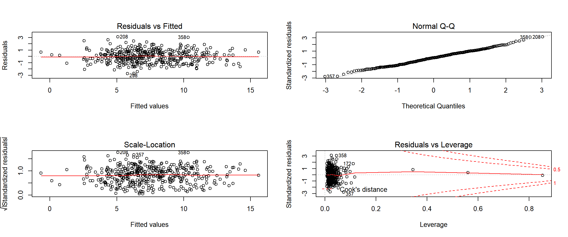
Conclusions
This notebook explored two datasets, Boston and Carseats, building multiple linear models for each.
The process was very similar for both datasets:
determine variable importance -> deal with collinearity -> dimension reduction -> add transforms/interactions -> assess
The results of following this process differed quite a bit between the two datasets, however. The Boston dataset responding very well to the transformed terms added, increasing the R-squared value significantly. The Carseats dataset was rather unresponsive to the applied transforms.
There could be several different reasons for the alternate outcomes, could be because one dataset was real and the other contrived, or because one had all continuous variables and the other had some categorical.
Future Work: A great deal more could be done with these datasets. For starters, a future task could be to try and make predictions with these models, adding more interactions or transforms to improve the R-squared values, stepping out of linear models and try using a GBM or RF to make more sense of the data, and more visualizations could be toyed with, expanding out into 3d or plotting on a map in the case of the Boston dataset.
References:
Code:
http://www-bcf.usc.edu/~gareth/ISL/ISLR%20Seventh%20Printing.pdf (Chap 3, sec 3.6.5-3.6.6)
Text:
https://stat.ethz.ch/R-manual/R-devel/library/MASS/html/Boston.html
https://www.cs.toronto.edu/~delve/data/boston/bostonDetail.html
https://cran.r-project.org/web/packages/ISLR/ISLR.pdf