Multi-Model Approach to Unbalanced Data with Caravan Dataset
Overview
This notebook will look at the 2016 Kaggle Caravan Insurance Challenge. The data was collected to see with the following goal in mind: > Can you predict who would be interested in buying a caravan insurance policy and give an explanation why?
Several models will be used in attempting to answer this question:
- Bagging
- Boosting (2 variants)
- Random Forest
As we are working with unbalanced data, each model will have be run against a training dataset in 4 different states: * Unbalanced (No modifications) * Undersampled * Oversampled * SMOTE * ROSE
Imports
library(tidyverse)
library(reshape2)
library(gridExtra)
library(caret) # Various models package
library(xgboost)
library(DMwR) # SMOTE
library(pROC) # ROC AUC Plotting
Data
The dataset used is from the CoIL Challenge 2000 datamining competition. It may be obtained from: https://www.kaggle.com/uciml/caravan-insurance-challenge
It contains information on customers of an insurance company. The data consists of 86 variables and includes product usage data and socio-demographic data derived from zip area codes.
A description of each variable may be found in data_dfns.md or at the link listed above.
Each number corresponds with a certain key, specific to each variable. There are 5 levels of keys, L0-L4 each key represents a different group range. As a sample:
L0 - Customer subtype (1-41)
    1: High Income, expensive child
    2: Very Important Provincials
    3: High status seniors
    ...
L1 - average age keys (1-6):
    1: 20-30 years
    2: 30-40 years
    3: 40-50 years
    ...
L2 - customer main type keys (1-10):
    1: Successful hedonists
    2: Driven Growers
    3: Average Family
    ...
L3 - percentage keys (0-9):
    0: 0%
    1: 1 - 10%
    2: 11 - 23%
    3: 24 - 36%
    ...
L4 - total number keys (0-9):
    0: 0
    1: 1 - 49
    2: 50 - 99
    3: 100 - 199
    ...
The variable descriptions are quite important as it appears as though the variable names themselves are abbreviated in Dutch. One helpful pattern to notice is the letters that variables begin with:
- M - primary demographics?, no guess for abbreviation
- A - numbers, possibly for dutch word aantal
- P - percents, possibly for dutch word procent
Acknowledgements
P. van der Putten and M. van Someren (eds) . CoIL Challenge 2000: The Insurance Company Case. Published by Sentient Machine Research, Amsterdam. Also a Leiden Institute of Advanced Computer Science Technical Report 2000-09. June 22, 2000.
head(cic <- read.csv('data/caravan-insurance-challenge.csv'), n=30)Exploratory Data Analysis
No NA values, all variables are type of int64. The data is peculiar in that every numeric value stands for an attribute of a person. Even variables that could be continuous, such as income, have been binned. In this sense, this dataset is entirely comprised of Categorical and Ordinal values. Other than potential collinearity between percentage and range values, the data is mostly clean.
For the EDA portion, we will cheat a bit and use knowledge from the combined dataset to get a better picture of the data. During the actual competition, contestants would not have had access to the CARAVAN variable where ORIGIN = train
cic %>% count(ORIGIN, CARAVAN)In both the given and hidden datasets we extremely imbalanced data. For every sample where caravan insurance was purchased, there are over 15 non-purchase cases. Attempting to run models without accounting for this descrepancy will surely impact the quality of our results.
# melt down a correlation matrix for plotting
cormat <- cic %>% subset(select=-c(ORIGIN)) %>% cor()
mcor <- cormat %>% melt()
mcor %>% ggplot(aes(x=Var1, y=Var2, fill=value)) +
geom_tile(color="white") +
scale_fill_gradient2(low= "blue", high = "red", mid = "white") +
theme(axis.text.x = element_text(angle = 90))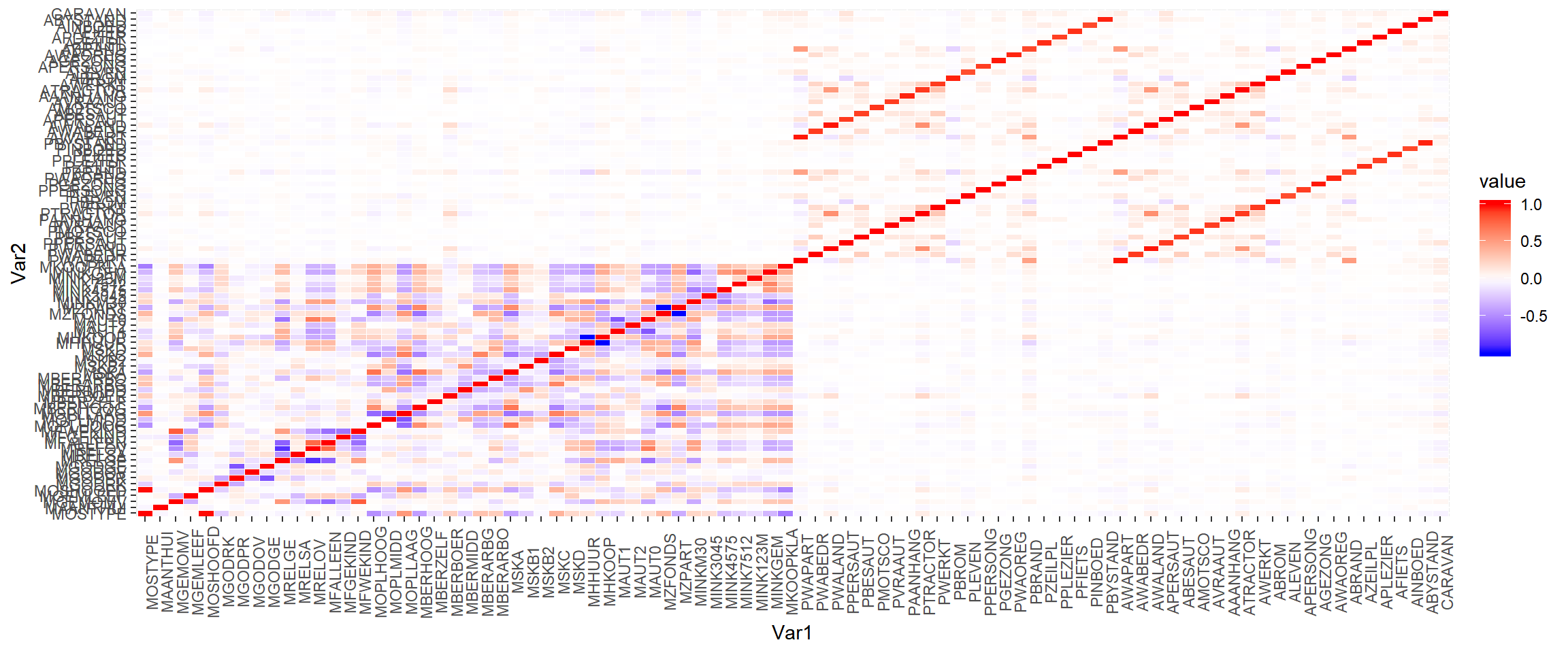
f43 <- unique(mcor$Var2)[0:43]

h1cor <- mcor %>% filter(Var1 %in% f43 & Var2 %in% f43)
h2cor <- mcor %>% filter(!(Var1 %in% f43) & !(Var2 %in% f43))

p1 <- h1cor %>%
  ggplot(aes(x=Var1, y=Var2, fill=value)) +
  ggtitle("Quadrant III") + geom_tile(color="white") +
  scale_fill_gradient2(low= "blue", high = "red", mid = "white") +
  theme(axis.text.x = element_text(angle = 90))

p2 <- h2cor %>%
  ggplot(aes(x=Var1, y=Var2, fill=value)) +
  ggtitle("Quadrant I") + geom_tile(color="white") +
  scale_fill_gradient2(low= "blue", high = "red", mid = "white") +
  theme(axis.text.x = element_text(angle = 90))

grid.arrange(p1, p2, nrow = 1)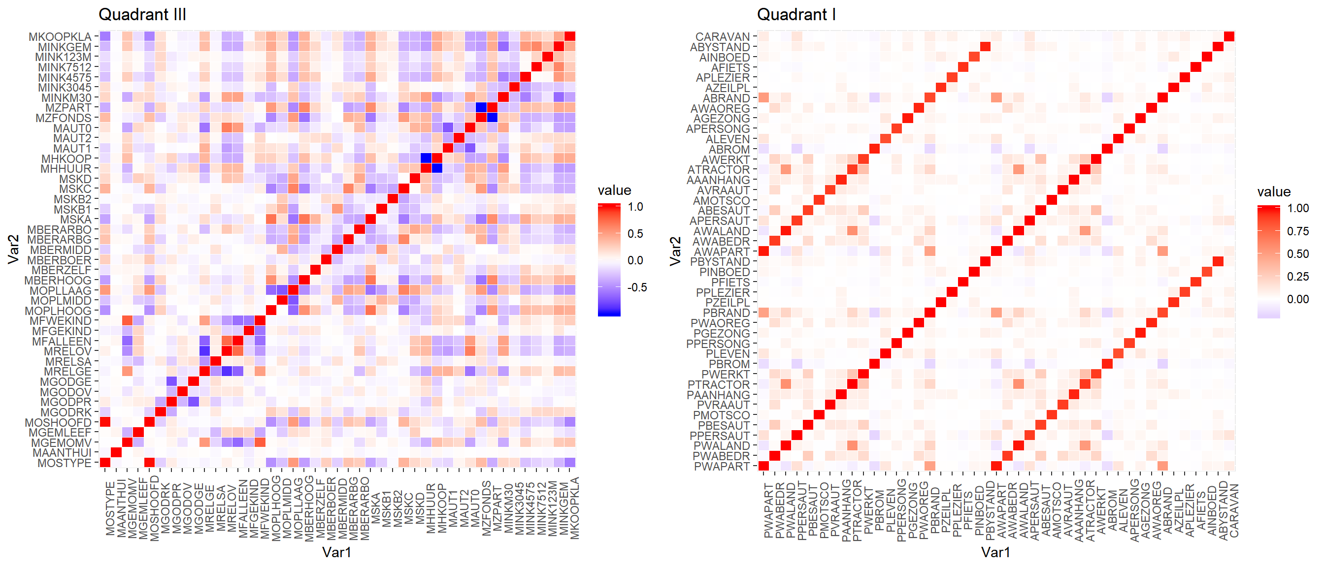
After zooming in a bit, the Quadrant I, L4 keys plot (right) shows how variables starting with P each have a corresponding variable starting with A this means that having both in our data will likely provide little value to the analysis.
Models
4 Models will be used in total: BaggingClassifier, RandomForestClassifier, AdaBoostClassifier from caret and xgboost
cic_data <- select(cic, -c(ORIGIN))
cic_data$CARAVAN <- factor(cic_data$CARAVAN, labels=c("No","Yes"))
Some models will not accept 0,1 as factor levels so assigning labels of No,Yes provides a quick work around. This will need to be undone for before using xgboost, as this model requires numeric levels for response variables.
# split data into train test
idx <- createDataPartition(cic_data$CARAVAN, p=0.75, list = FALSE)
train_data <- cic_data[idx,]
test_data <- cic_data[-idx,]
down_train <- downSample(x=select(train_data,-c(CARAVAN)), y=train_data$CARAVAN, yname="CARAVAN")
up_train <- upSample(x=select(train_data,-c(CARAVAN)), y=train_data$CARAVAN, yname="CARAVAN")
smote_train <- SMOTE(CARAVAN ~., data = train_data)
#rose_train <- ROSE(CARAVAN ~., data = train_data)$data
props <- data.frame(bind_rows(table(train_data$CARAVAN),
table(down_train$CARAVAN),
table(up_train$CARAVAN),
table(smote_train$CARAVAN)),
#table(rose_train$CARAVAN)),
row.names = c('Unbalanced','Downsample','Upsample','SMOTE'))
props$Total <- props$No+props$Yes
propsWe can see here how the various methods of resampling affected the training data proportions. Only upsampling increased the size of the training set, all others used a decreasing or size maintaining rebalancing approach.
- Random Downsampling
- Random Upsampling
- SMOTE
ROSE - Random Over-Sampling Examples, produces a synthetic, possibly balanced, sample of data simulated according to a smoothed-bootstrap approach. This approach is similar to SMOTE in that it entirely new data is created rather than simply randomly sampling from the existing data.
ROSE was previously included, but the algorithms usefulness has been debated and for this particular dataset, it consistantly performed far worse than the other three methods.
cfmROC <- function(y_pred, y_true){

  cm <- confusionMatrix(y_pred, y_true)
  rocobj <- roc(as.numeric(y_true)-1, as.numeric(y_pred)-1)

  # Plot ROC AUC
  p1 <- ggroc(rocobj, alpha = 0.5, colour = "red", linetype = 2, size = 2) +
    geom_line(aes(x = rocobj$thresholds, y = rev(rocobj$thresholds))) +
    geom_text(aes(x = 0.25, y = 0.25), label = paste("AUC:",round(rocobj$auc,4))) +
    ggtitle("ROC curve")

  # Plot confusion matrix
  p2 <- cm$table %>% as.data.frame() %>%
    ggplot(aes(x = Reference, y = Prediction)) +
    geom_tile(aes(fill = log(Freq)), colour = "white") +
    scale_fill_gradient(low = "white", high = "steelblue") +
    geom_text(aes(x = Reference, y = Prediction, label = Freq)) +
    theme(legend.position = "none") +
    ggtitle(paste("Accuracy", signif(cm$overall[1], digits = 4), "| Kappa", signif(cm$overall[2], digits = 4)))

  grid.arrange(grobs = list(p2, p1),widths = c(1, 1.2))
}
run.xgb <- function(traind, testd){
# Convert dataframe -> matrix, factors -> numeric (0,1)
mat_train <- as.matrix(subset(traind, select=-c(CARAVAN)))
clabel <- (as.numeric(as.factor(traind$CARAVAN)) - 1)
dtrain <- xgb.DMatrix(data = mat_train, label = clabel)
# Train model on converted training data
bstDMatrix <- xgboost(data = dtrain, max.depth = 3, eta = 1, nthread = 4, nrounds = 2, objective = "binary:logistic")
# Convert test data into compatable matrix, numeric format
mat_test <- as.matrix(subset(testd, select=-CARAVAN))
clabel_test <- (as.numeric(as.factor(testd$CARAVAN)) - 1)
dtest <- xgb.DMatrix(data = mat_test, label = clabel_test)
# Predict test data and convert to binary output
preds_x <- predict(bstDMatrix, dtest)
preds_x.bin <- as.factor(ifelse(preds_x > 0.5, 1, 0))
# Plot confusion matrix and ROC AUC
cfmROC(preds_x.bin, as.factor(clabel_test))
return(bstDMatrix)
}run.model <- function(method="rf", traind, testd){
# XGBoost is a seperate package from caret, so we modifiy our wrapper function to pass it to run.xgb
if (method=="xgb") return(run.xgb(traind, testd))
mod <- train(CARAVAN ~ ., data = traind,
method = method,
metric = "ROC",
preProcess = c("scale", "center"),
trControl = ctrl)
pred <- predict(mod, subset(testd, select=-CARAVAN))
cfmROC(pred, testd$CARAVAN)
return(mod)
}Defining a few helper functions drastically reduces the amount of repeatitious code required. The caret package makes this very easy for us by accepting nearly identical baseline parameters for all models.
ctrl <- trainControl(method = "none", classProbs = TRUE)This will serve as the baseline training control for all models. Setting method to “none” disables cross validation, we could certainly build better models with CV enabled, but it significantly increases training time, later notebooks will explore this in detail. Setting classProbs=TRUE gives us probabilities rather than binary outputs and so that ROC may be used as our evaluation metric.
Unbalanced
To establish a frame of reference, we will first try running all four models against the original data, making to attempts to correct the imbalance.
Bagging
bag_orig <- train(CARAVAN ~ ., data = train_data,
                  method = "treebag",
                  metric = "ROC",
                  preProcess = c("scale", "center"),
                  trControl = ctrl)

preds <- predict(bag_orig, subset(test_data, select=-CARAVAN))
head(preds)
## [1] No No No No No No
## Levels: No YesIt is all too easy to be mislead by a high accuracy score, 91.6% would be quite good if we were dealing with balanced data, but with this set being as imbalanced as it is, this score is actually worse than if the model had just chosen 0(‘No’) for every sample, taking this route would have yielded ~94% accuracy.
cfmROC(preds,test_data$CARAVAN)
Boosting (Adaboost)
ada_orig <- train(CARAVAN ~ ., data = train_data,
                  method = "ada",
                  metric = "ROC",
                  preProcess = c("scale", "center"),
                  trControl = ctrl)

pred <- predict(ada_orig, subset(test_data, select=-CARAVAN))

cfmROC(pred, test_data$CARAVAN)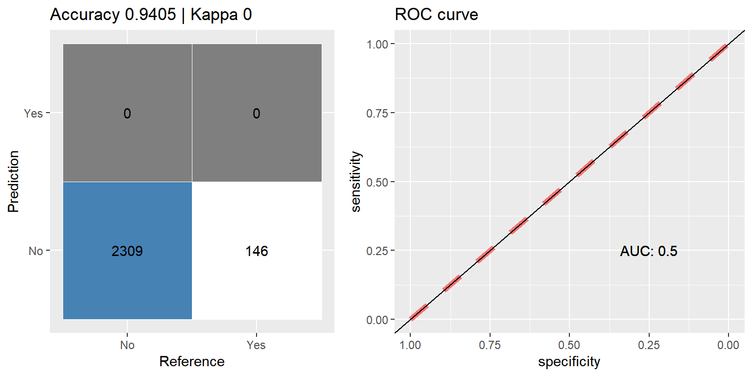
Random Forest
rf_orig <- train(CARAVAN ~ ., data = train_data,
                      method = "rf",
                      metric = "ROC",
                      preProcess = c("scale", "center"),
                      trControl = ctrl)

pred <- predict(rf_orig, subset(test_data, select=-CARAVAN))
cfmROC(pred, test_data$CARAVAN)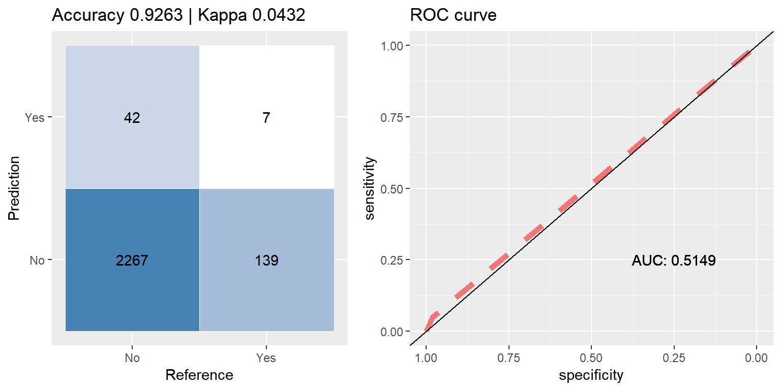
XGBoost
mat_train <- as.matrix(subset(train_data,select=-CARAVAN))
c_label <- (as.numeric(as.factor(train_data$CARAVAN)) - 1)
XGBoost requires matrices rather than data.frames for inputs. It also requiress binary response variables (0,1) rather than factors. R is 1 indexed rather than 0 indexed, so subtracting 1 from a numeric convertion achieves these requirements.
dtrain <- xgb.DMatrix(data = mat_train, label = c_label)

xgb_orig <- xgboost(data = dtrain,
                      max.depth = 3,
                      eta = 1, # learning rate
                      nthread = 4, # multithreading support
                      nrounds = 2,
                      objective = "binary:logistic")
## [1] train-error:0.059183
## [2] train-error:0.059454# Preform the same transformations on the test data
mat_test <- as.matrix(subset(test_data,select=-CARAVAN))
c_label_test <- (as.numeric(as.factor(test_data$CARAVAN)) - 1)
dtest <- xgb.DMatrix(data = mat_test, label = c_label_test)
preds_xgb <- predict(xgb_orig, dtest)# convert xgb's predicted probabilities back into binary output
cfmROC(as.factor(ifelse(preds_xgb > 0.5, 1, 0)), as.factor(c_label_test))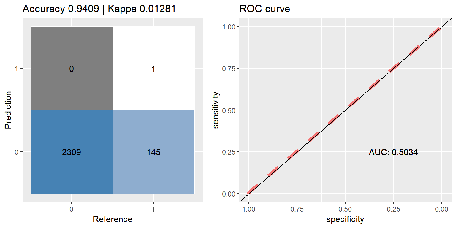
Downsampling
Random Downsampling - balances data by randomly under under selecting from the majority class, those who did not purchase caravan insurance.
Bagging
bag_down <- train(CARAVAN ~ ., data = down_train,
                      method = "treebag",
                      metric = "ROC",
                      preProcess = c("scale", "center"),
                      trControl = ctrl)

pred <- predict(bag_down, subset(test_data, select=-CARAVAN))
cfmROC(pred,test_data$CARAVAN)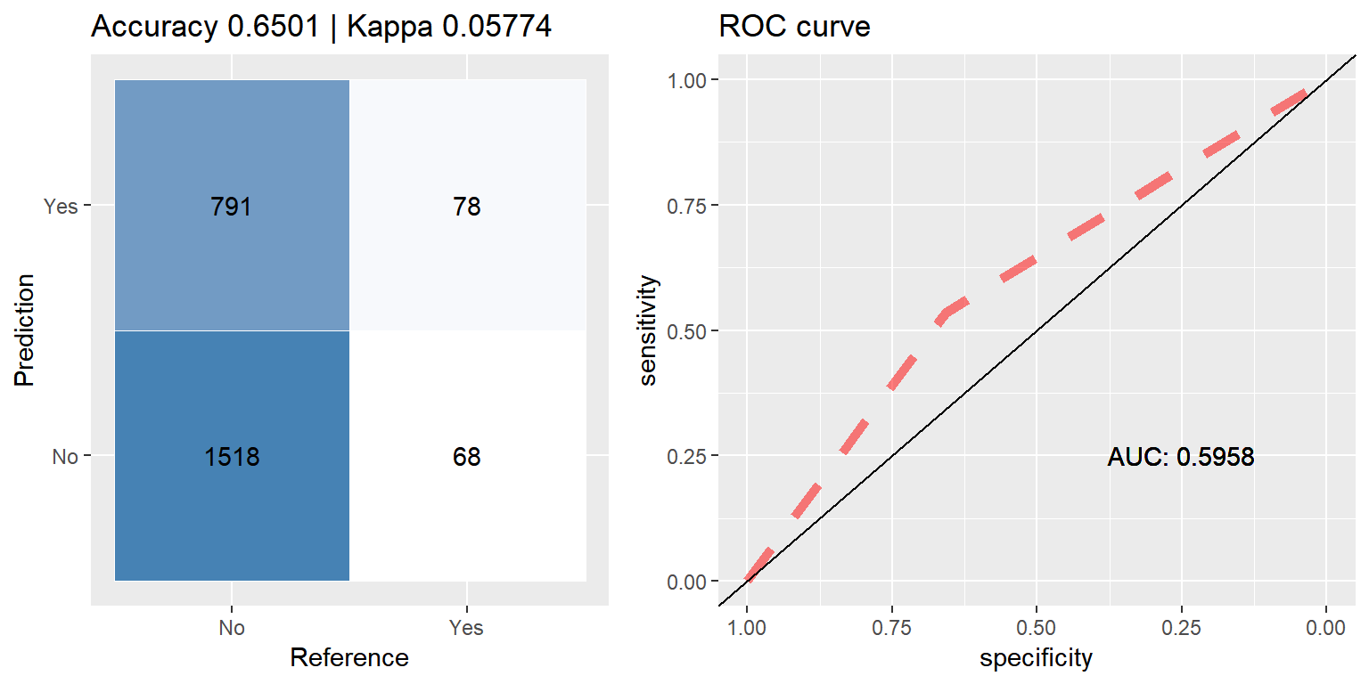
The only change moving between data resamplings is the data = .. parameter, every other will be fixed constant. Hereafter, we can use the nice little wrapper function run.model to help keep us DRY.
Boosting (Adaboost)
ada_down <- run.model(method = "ada", traind = down_train, testd = test_data)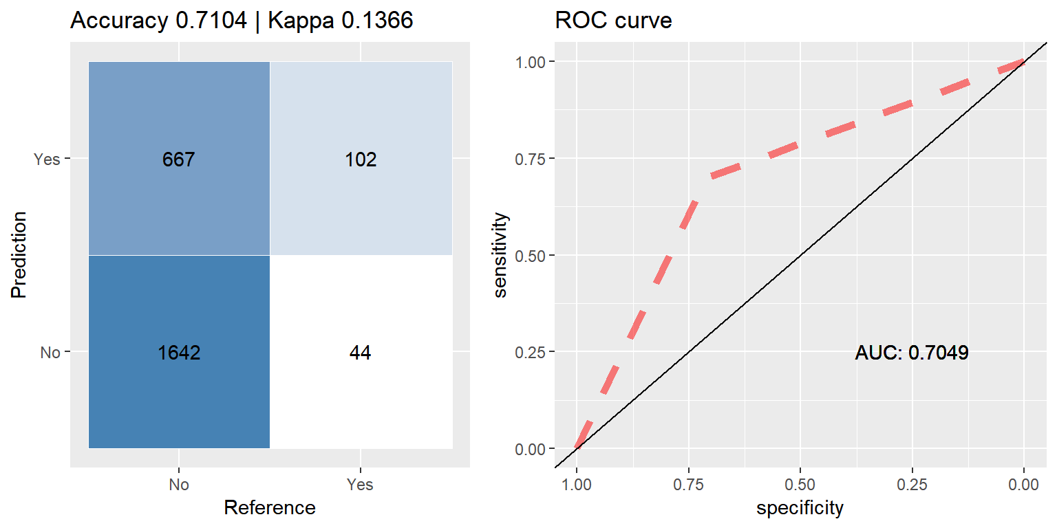
Random Forest
rf_down <- run.model(method = "rf", traind = down_train, testd = test_data)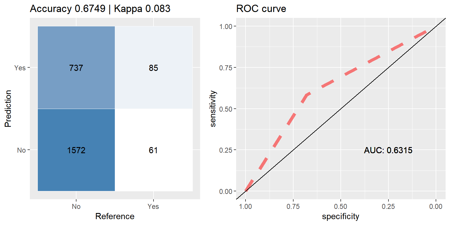
XGBoost
xgb_down <- run.model(method = "xgb", traind = down_train, testd = test_data)## [1] train-error:0.332955
## [2] train-error:0.286364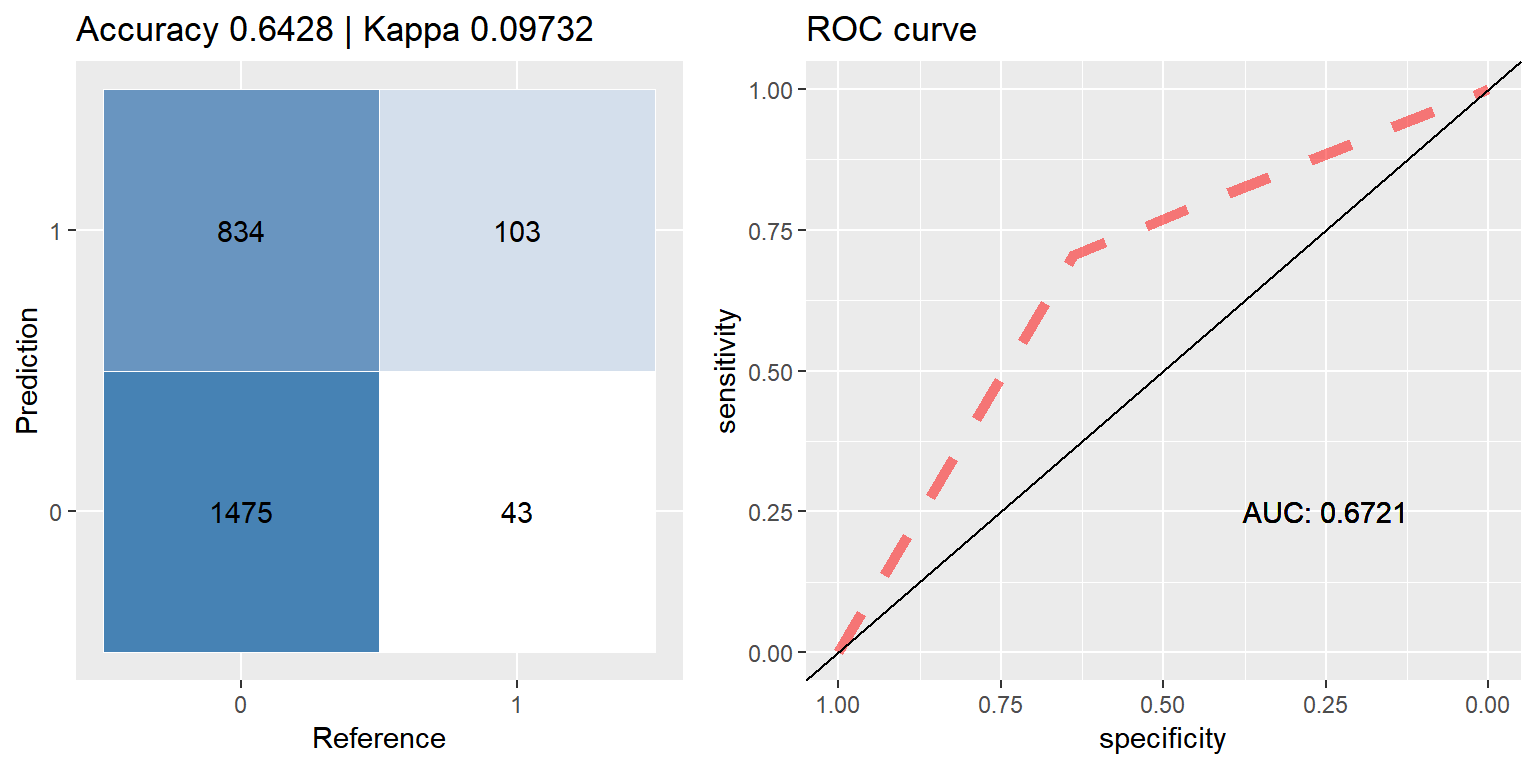
Upsampling
Random Upsampling - attempts to balance the data by randomly selecting from the minority class, in this case, those who did purchase a caravan insurance policy.
Bagging
bag_up <- run.model(method = "treebag", up_train, test_data)
Boosting (Adaboost)
ada_up <- run.model(method = "ada", up_train, test_data)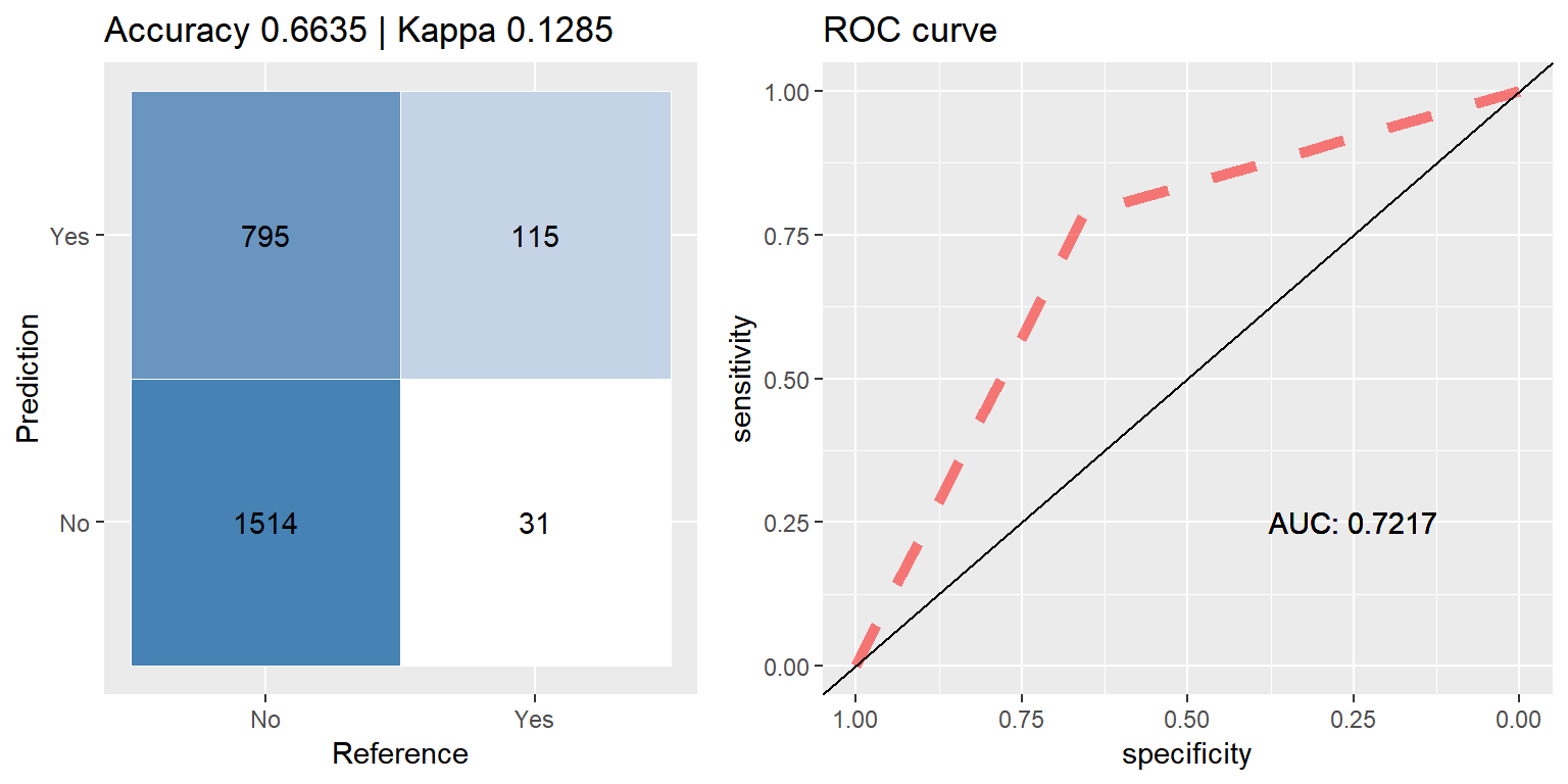
Random Forest
rf_up <- run.model(method = "rf", up_train, test_data)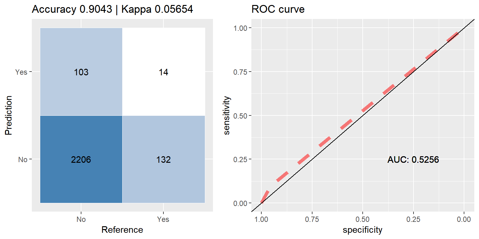
XGBoost
xgb_up <- run.model(method = "xgb", up_train, test_data)## [1] train-error:0.317814
## [2] train-error:0.305688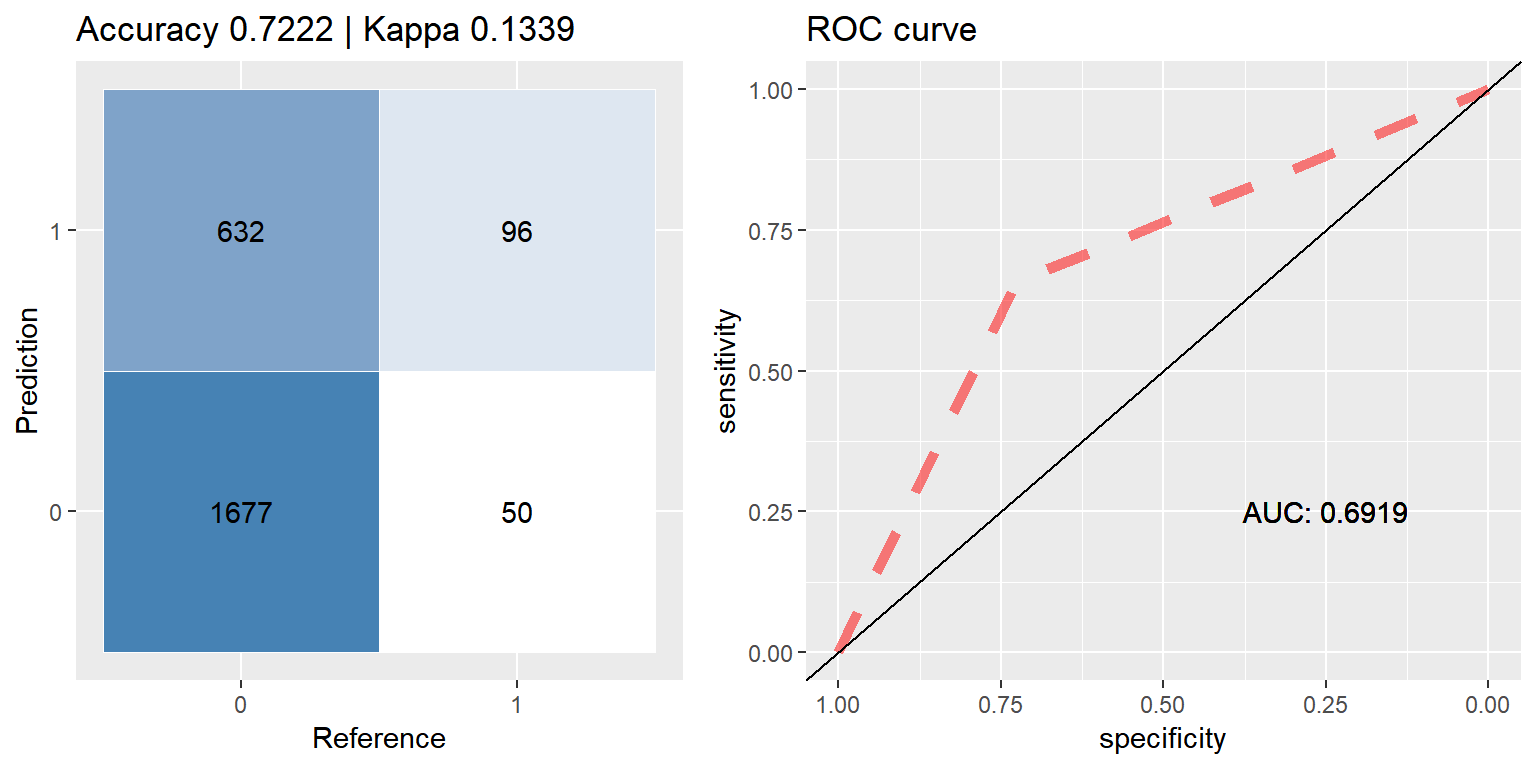
SMOTE
SMOTE - Synthetic Minority Over-sampling Technique, constructs new synthetic data by sampling neighboring points. Balancing happens through both oversampling the minority and undersampling the major class.
Bagging
bag_smote <- run.model(method = "treebag", smote_train, test_data)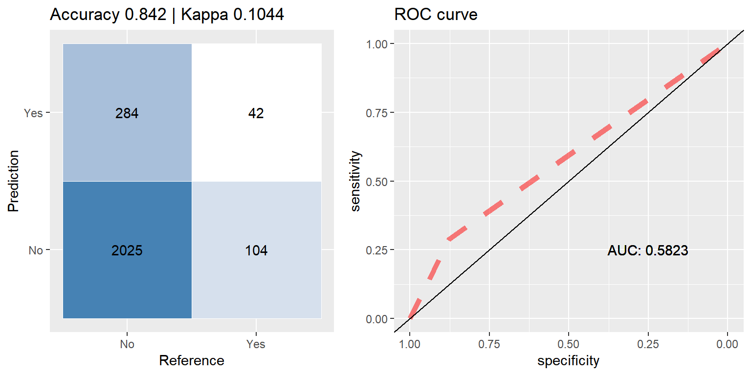
Boosting (Adaboost)
ada_smote <- run.model(method = "ada", smote_train, test_data)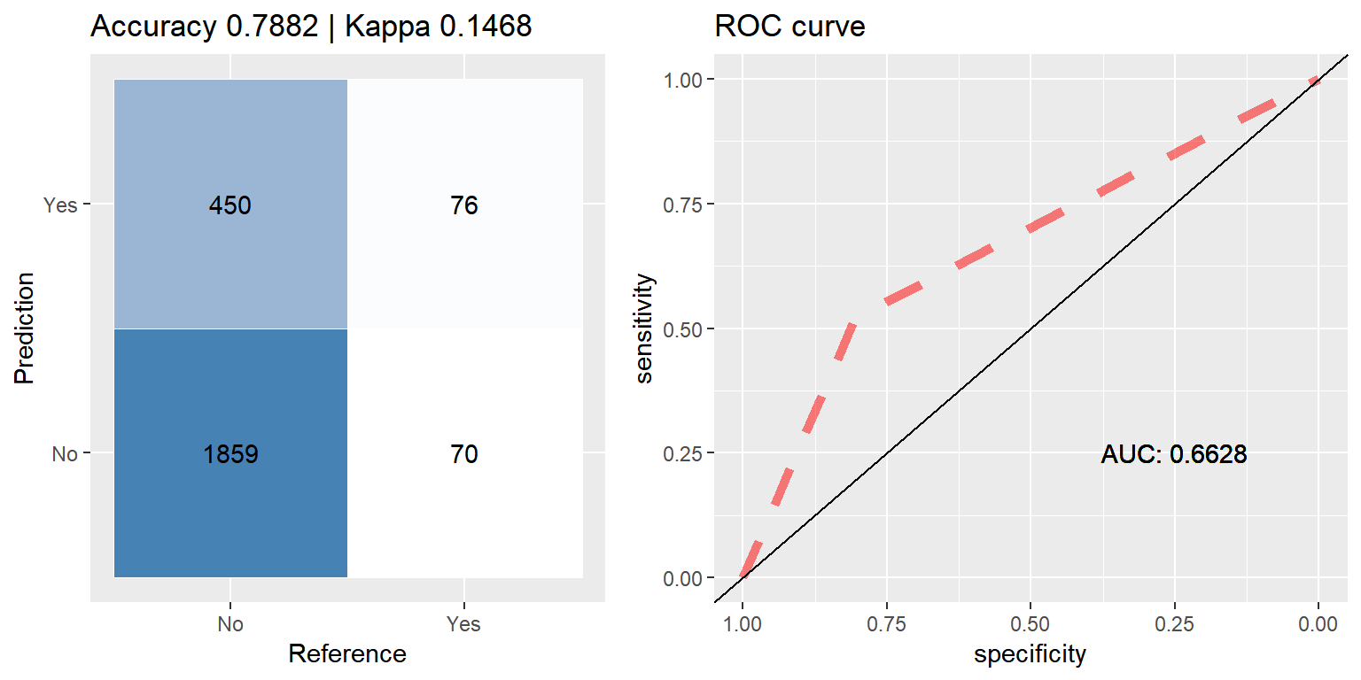
Random Forest
rf_smote <- run.model(method = "rf", smote_train, test_data)
XGBoost
xgb_smote <- run.model(method = "xgb", smote_train, test_data)## [1] train-error:0.234091
## [2] train-error:0.183117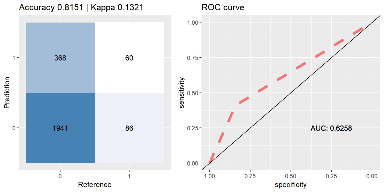
Feature Importance
bag_orig.imp <- varImp(bag_orig, scale=FALSE)
ada_orig.imp <- varImp(ada_orig, scale = FALSE)
rf_orig.imp <- varImp(rf_orig, scale=FALSE)
xgb_orig.imp <- xgb.importance(model = xgb_orig)
library(docstring)
get.imps <- function(models = list(bag,ada,rf,xgb)){
#' Calculates feature importances
#'
#' Calculates and returns all 4 models' feature importances
#'
#' @param models a list of models to calculate feature importance. Must be exactly in parameter order specified
caret.imps <- lapply(models[1:3], varImp, scale=FALSE)
imps <- lapply(caret.imps, getElement, name='importance')
imps[[4]] <- xgb.importance(model = models[[4]])
return(imps)
}plot.featimps <- function(resample.method="Unbalanced"){
#' Plot feature importances
#'
#' Plots all four models feature importances
#'
#' @param resample.method model set to use: ("Unbalanced" | "Downsampled" | "Upsampled" | "SMOTE")
#'
if(grepl("(unb|ori).*",resample.method,ignore.case = TRUE)){
resample.method <- "Unbalanced"
imps <- get.imps(list(bag_orig, ada_orig, rf_orig, xgb_orig))
}else if(grepl("(und|dow).*",resample.method, ignore.case = TRUE)){
resample.method <- "Downsampled"
imps <- get.imps(list(bag_down, ada_down, rf_down, xgb_down))
}else if(grepl("(up|ove).*",resample.method, ignore.case = TRUE)){
resample.method <- "Upsampled"
imps <- get.imps(list(bag_up, ada_up, rf_up, xgb_up))
}else if(grepl("sm.*",resample.method, ignore.case = TRUE)){
resample.method <- "SMOTE"
imps <- get.imps(list(bag_smote, ada_smote, rf_smote, xgb_smote))
} else stop("invalid resample selection ('orig'|'down'|'up'|'smote')")
# resample.method <- ifelse(grepl("(unba|ori).+",resample.method,ignore.case = TRUE),"Unbalanced",resample.method)
# resample.method <- ifelse(grepl("(und|dow).+",resample.method, ignore.case = TRUE),"Downsampled",resample.method)
# resample.method <- ifelse(grepl("(up|ove).+",resample.method, ignore.case = TRUE),"Upsampled",resample.method)
# resample.method <- ifelse(grepl("sm.+",resample.method, ignore.case = TRUE),"SMOTE",resample.method)
# imps <- switch (resample.method,
# Unbalanced = get.imps(list(bag_orig, ada_orig, rf_orig, xgb_orig)),
# Downsampled = get.imps(list(bag_down, ada_down, rf_down, xgb_down)),
# Upsampled = get.imps(list(bag_up, ada_up, rf_up, xgb_up)),
# SMOTE = get.imps(list(bag_smote, ada_smote, rf_smote, xgb_smote))
# )
# Bagging
p1 <- imps[[1]] %>%
transmute(Feature=as.factor(row.names(imps[[1]])),Importance=Overall ) %>%
top_n(10) %>%
ggplot(aes(x=reorder(Feature,Importance), fill=Feature, weight=Importance)) +
geom_bar() +
coord_flip() +
theme(legend.position="none") +
labs(x="Feature", y=NULL, title=paste("Bagging",resample.method))
# Boosting
p2 <- imps[[2]] %>%
transmute(Feature=as.factor(row.names(imps[[2]])),Importance=((No+Yes)-1)) %>%
top_n(10) %>%
ggplot(aes(x=reorder(Feature,Importance), fill=Feature, weight=Importance)) +
geom_bar() +
coord_flip() +
theme(legend.position="none") +
labs(x=NULL, y=NULL, title=paste("Boosting (Ada)",resample.method))
# Random Forest
p3 <- imps[[3]] %>%
transmute(Feature=as.factor(row.names(imps[[3]])),Importance=Overall/100) %>%
top_n(10) %>%
ggplot(aes(x=reorder(Feature,Importance), fill=Feature, weight=Importance)) +
geom_bar() +
coord_flip() +
theme(legend.position="none") +
labs(x="Feature", y="Importance", title=paste("Random Forest",resample.method))
#XGBoost
p4 <- xgb.ggplot.importance(imps[[4]]) +
geom_col(aes(width=0.8, fill=Cluster)) +
labs(x=NULL, y="Importance", title=paste("XGBoost",resample.method)) +
theme(plot.title = element_text(face="plain"))
grid.arrange(p1,p2,p3,p4, layout_matrix=rbind(c(1,2),c(3,4)))
}grepl("sm.+","smt", ignore.case = TRUE)## [1] TRUEplot.featimps("Unbalanced")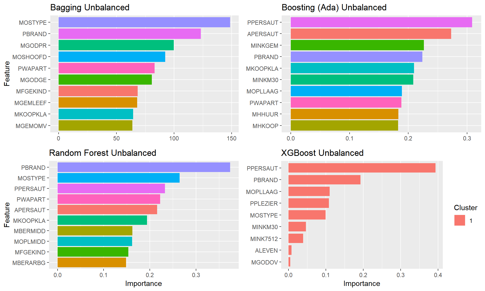
plot.featimps("Down")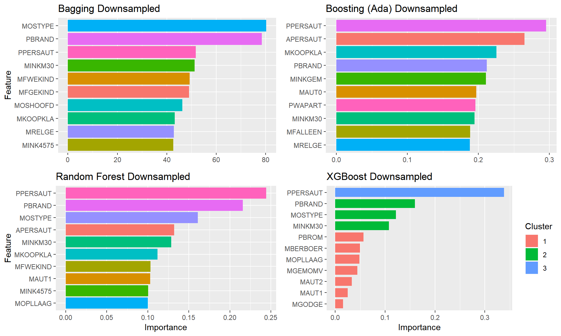
plot.featimps("Up")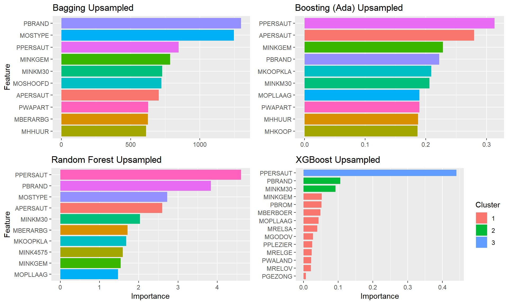
plot.featimps("SMOTE")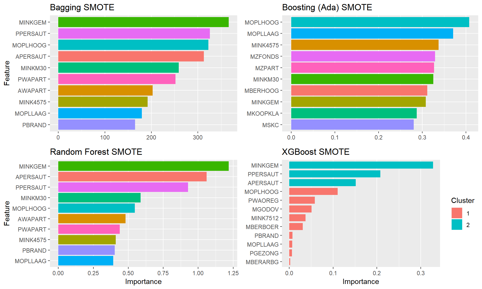
Conclusions
In this notebook, we explored the CoIL Challenge 2000 datamining competition dataset. 4 Different models were used:
A BaggingClassifer, AdaBoost, Random Forrest, and XGBoost.
For each of these models, we 4 variants of the same training dataset:
Unaltered, Undersampled, Oversampled, and SMOTE.
We determined that without altering the data, the ROC score is no better than randomly guessing, Oversampling and SMOTE performed slightly better, but Undersampling was clearly the best approach.
After testing each model with the data modifications, a brute force method of Hyperparameter tuning was attempted via GridSearch followed by an automated means of feature selection. Neither of these methods yielded substantially better results for the compute time they required.
The highest end ROC score we were able to achieve in the synthetic competition environment was 0.66 with a overtuned Random Forest. The highest local test score was 0.784, showing that the model was clearly beginning to overfit the data.
At this time, I am unable to answer the question of: > Who is interested in buying Caravan Insurance and why?
with any degree of certainty. The winner of the 2000 challenge determined the strongest indicators variables were number of car policies, buying power, and various other policies held.
Future work: Countless parameters have been left untweaked, each model could have it’s own grid search with each hyperparameter explored. As mentioned earlier, there was an issue with collinearity between percentage variables and number variables, this should be explored further. There is a great deal of EDA left undone, deeper relationships between variables should be investigated through interactions and transformations. Additionally, since this dataset is comprised largely of categorical variables, ordinal or otherwise, CatBoost might be a pragmatic choice for modeling, even attempting to use a Neural Network may yield interesting results.
References
Code & Docs
https://shiring.github.io/machine_learning/2017/04/02/unbalanced
https://topepo.github.io/caret/subsampling-for-class-imbalances.html
https://amunategui.github.io/binary-outcome-modeling/
http://dpmartin42.github.io/posts/r/imbalanced-classes-part-1
https://cran.r-project.org/web/packages/egg/vignettes/Ecosystem.html
Text:
https://www.kaggle.com/uciml/caravan-insurance-challenge/home
Definitions
http://glemaitre.github.io/imbalanced-learn/generated/imblearn.over_sampling.RandomOverSampler.html
http://glemaitre.github.io/imbalanced-learn/generated/imblearn.over_sampling.SMOTE.html
Other:
https://web.archive.org/web/20160818233319/http://www.wi.leidenuniv.nl/~putten/library/cc2000/
https://github.com/jayanttikmani/cross-sellingCaravanInsuranceUsingDataMining/
https://www.statmethods.net/input/valuelabels.html
https://campus.datacamp.com/courses/free-introduction-to-r/chapter-4-factors-4?ex=4
https://stackoverflow.com/questions/5869539/confusion-between-factor-levels-and-factor-labels