Gradient Boosting with XGBoost and the Agaricus Dataset
Overview
This notebook will take a look at agaricus dataset (Mushroom Database) originally drawn from The Audubon Society Field Guide to North American Mushrooms and hosted in the UCI Machine Learning Repository.
The goal is to create model that can accurately differentiate between edible and poisonous mushrooms.
To do this two models will be used: * sklearn’s RandomForestClassifer * XGBoost’s XGBClassifier
Each model will be used on both a simple numeric mapping and a one-hot encoding of the dataset. In addition to model performance, feature importances will be examined for each model and decision trees built when possible.
Imports
library(tidyverse)
library(xgboost)
library(caret)
library(ranger) # fast Random Forest
library(mltools) # onehot encoding
library(data.table)
Data
The dataset may be obtained from:
https://archive.ics.uci.edu/ml/datasets/mushroom or https://www.kaggle.com/uciml/mushroom-classification
Additionally, a dataset is used from the XGBoost repository which can be found here:
https://github.com/dmlc/xgboost/tree/master/demo/data
The Kaggle link is preferred simply for convenience as the columns have already been labeled with sensible names.
This dataset includes descriptions of hypothetical samples corresponding to 23 species of gilled mushrooms in the Agaricus and Lepiota Family Mushroom drawn from The Audubon Society Field Guide to North American Mushrooms (1981). Each species is identified as definitely edible, definitely poisonous, or of unknown edibility and not recommended. This latter class was combined with the poisonous one.
Each entry in dataset contains only a single letter, a reference table containing corresponding meanings can be found in data/agaricus-lepiota.names or at https://archive.ics.uci.edu/ml/machine-learning-databases/mushroom/agaricus-lepiota.names
data(agaricus.train, package='xgboost')
data(agaricus.test, package='xgboost')
train <- agaricus.train
test <- agaricus.testglimpse(train)## List of 2
## $ data :Formal class 'dgCMatrix' [package "Matrix"] with 6 slots
## .. ..@ i : int [1:143286] 2 6 8 11 18 20 21 24 28 32 ...
## .. ..@ p : int [1:127] 0 369 372 3306 5845 6489 6513 8380 8384 10991 ...
## .. ..@ Dim : int [1:2] 6513 126
## .. ..@ Dimnames:List of 2
## .. ..@ x : num [1:143286] 1 1 1 1 1 1 1 1 1 1 ...
## .. ..@ factors : list()
## $ label: num [1:6513] 1 0 0 1 0 0 0 1 0 0 ...XGBoost includes the agaricus dataset by default as example data. To keep it small, they’ve represented the set as a sparce matrix. This is a fantastic way to limit the size of a dataset, but it isn’t exactly easily interperatable.
# Same dataset, but with legible names
head(agar <- read.csv('data/mushrooms.csv'))
The kaggle provided dataset is much more human friendly, providing factor codes for each column.
Exploratory Data Analysis
Short of one variable having with NA values, this dataset is quite clean. It is entirely comprised of categorical values, each with a relatively low cardinality. It is slightly imbalanced, having 4208 (51.8%) entries marked as edible and 3916 (48.2%) marked poisonous, a small discrepancy, but it shouldn’t significantly affect our model.
dim(train$data)## [1] 6513 126dim(test$data)## [1] 1611 126head(train$data, n=10)## [1] 0 0 1 0 0 0 1 0 1 0str(agar)## 'data.frame': 8124 obs. of 23 variables:
## $ class : Factor w/ 2 levels "e","p": 2 1 1 2 1 1 1 1 2 1 ...
## $ cap.shape : Factor w/ 6 levels "b","c","f","k",..: 6 6 1 6 6 6 1 1 6 1 ...
## $ cap.surface : Factor w/ 4 levels "f","g","s","y": 3 3 3 4 3 4 3 4 4 3 ...
## $ cap.color : Factor w/ 10 levels "b","c","e","g",..: 5 10 9 9 4 10 9 9 9 10 ...
## $ bruises : Factor w/ 2 levels "f","t": 2 2 2 2 1 2 2 2 2 2 ...
## $ odor : Factor w/ 9 levels "a","c","f","l",..: 7 1 4 7 6 1 1 4 7 1 ...
## $ gill.attachment : Factor w/ 2 levels "a","f": 2 2 2 2 2 2 2 2 2 2 ...
## $ gill.spacing : Factor w/ 2 levels "c","w": 1 1 1 1 2 1 1 1 1 1 ...
## $ gill.size : Factor w/ 2 levels "b","n": 2 1 1 2 1 1 1 1 2 1 ...
## $ gill.color : Factor w/ 12 levels "b","e","g","h",..: 5 5 6 6 5 6 3 6 8 3 ...
## $ stalk.shape : Factor w/ 2 levels "e","t": 1 1 1 1 2 1 1 1 1 1 ...
## $ stalk.root : Factor w/ 5 levels "?","b","c","e",..: 4 3 3 4 4 3 3 3 4 3 ...
## $ stalk.surface.above.ring: Factor w/ 4 levels "f","k","s","y": 3 3 3 3 3 3 3 3 3 3 ...
## $ stalk.surface.below.ring: Factor w/ 4 levels "f","k","s","y": 3 3 3 3 3 3 3 3 3 3 ...
## $ stalk.color.above.ring : Factor w/ 9 levels "b","c","e","g",..: 8 8 8 8 8 8 8 8 8 8 ...
## $ stalk.color.below.ring : Factor w/ 9 levels "b","c","e","g",..: 8 8 8 8 8 8 8 8 8 8 ...
## $ veil.type : Factor w/ 1 level "p": 1 1 1 1 1 1 1 1 1 1 ...
## $ veil.color : Factor w/ 4 levels "n","o","w","y": 3 3 3 3 3 3 3 3 3 3 ...
## $ ring.number : Factor w/ 3 levels "n","o","t": 2 2 2 2 2 2 2 2 2 2 ...
## $ ring.type : Factor w/ 5 levels "e","f","l","n",..: 5 5 5 5 1 5 5 5 5 5 ...
## $ spore.print.color : Factor w/ 9 levels "b","h","k","n",..: 3 4 4 3 4 3 3 4 3 3 ...
## $ population : Factor w/ 6 levels "a","c","n","s",..: 4 3 3 4 1 3 3 4 5 4 ...
## $ habitat : Factor w/ 7 levels "d","g","l","m",..: 6 2 4 6 2 2 4 4 2 4 ...str() truly is a powerful tool, there are 3 primary things are worth noting here:
- The highest caridinality we see in any single column is 12 for
gill.color. stalk.rootcontains “?” as one of its factors, likely representing a missing valueveil.typeonly has a single value, meaning that it will contribute nothing to our classification models.
agar.dt <- agar %>% as.data.table() %>% select(-c(veil.type))
head(agar.oh <- one_hot(agar.dt, cols = colnames(subset(agar.dt, select = -class))))
agar.oh$class <- as.factor(as.numeric(agar.oh$class)-1) # Denote (p)osionious = 1, (e)atible = 0
setnames(agar.oh, old=c("stalk.root_?"), new=c("stalk.root_NA"))library(corrplot)
colo<- colorRampPalette(c("blue", "white", "red"))(200)
corrplot(cor(data.matrix(agar.dt)), col = colo)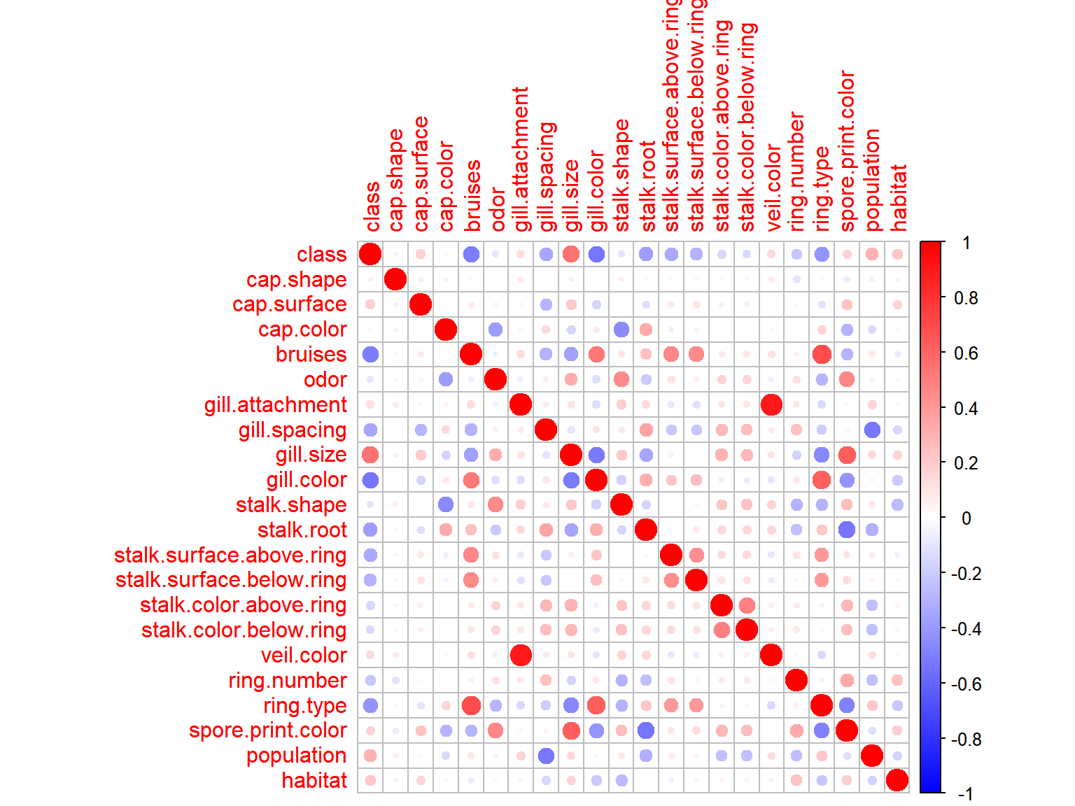
Two variable pairs have extremely strong correlations with one another, veil.color + gill.attachment and ring.type + bruises. There are also quite a few features that correlate rather strongly with the response variable, these will be worth keeping in mind durring the later stages of analysis.
Models
Random Forest
ttidx <- createDataPartition(agar.oh$class,p=0.70,list = F)
agar.test <- agar.oh[!ttidx]
agar.train <- agar.oh[ttidx]
#setnames(agar.train, old=c("stalk.root_?"), new=c("stalk.root_NA"))
#setnames(agar.test, old=c("stalk.root_?"), new=c("stalk.root_NA"))#train(class~., data = agar.train, method="rf", trControl=trainControl(method="cv", number=5)) # caret's rf
model.rf <- ranger(class~., data = agar.train, importance = "impurity")Using the ranger library rather than caret’s Random Forest implementation reduced the run time from several minutes to ~2 seconds.
preds.rf <- predict(model.rf, data = agar.test)
confusionMatrix(preds.rf$predictions, agar.test$class)
## Confusion Matrix and Statistics
##
## Reference
## Prediction 0 1
## 0 1262 0
## 1 0 1174
##
## Accuracy : 1
## 95% CI : (0.9985, 1)
## No Information Rate : 0.5181
## P-Value [Acc > NIR] : < 2.2e-16
##
## Kappa : 1
##
## Mcnemar's Test P-Value : NA
##
## Sensitivity : 1.0000
## Specificity : 1.0000
## Pos Pred Value : 1.0000
## Neg Pred Value : 1.0000
## Prevalence : 0.5181
## Detection Rate : 0.5181
## Detection Prevalence : 0.5181
## Balanced Accuracy : 1.0000
##
## 'Positive' Class : 0
## Using no fancy tricks, no model tuning, we end up with a perfect classification. Now, whenever we see a model perform perfect classification, as a good data scientist, the first thing one should think is “oh no, what did I do wrong..”
So, let’s dig in to the model and see if we can learn a bit more about how this scenario came to be. A couple common things to check for could be: * Was any overlap introduced between training and test set? * Could there be data leakage between the response variable and any of the features? * Was the testing set substainly less complicated than the training set?
imps.rf <-setnames(setDT(data.frame(importance = importance(model.rf)), keep.rownames = TRUE)[], 1, "feature")
imps.rf$feature <- as.factor(imps.rf$feature)
To start off, let’s have a look at which features were determined to be important by the Random Forest model.
imps.rf %>%
  mutate(featgrp=strsplit(as.character(imps.rf$feature),"_") %>% lapply(`[[`, 1)%>% unlist()) %>%
  top_n(35,wt=importance) %>%
  ggplot(aes(x=reorder(feature,desc(importance)), fill=as.factor(featgrp), weight=importance)) +
  geom_bar() +
  theme(legend.position="none", axis.text.x = element_text(angle = 90, hjust = 1)) +
  labs(x="Feature", y="Importance", title="ranger Gini impurity feature importance (colored by parent group)")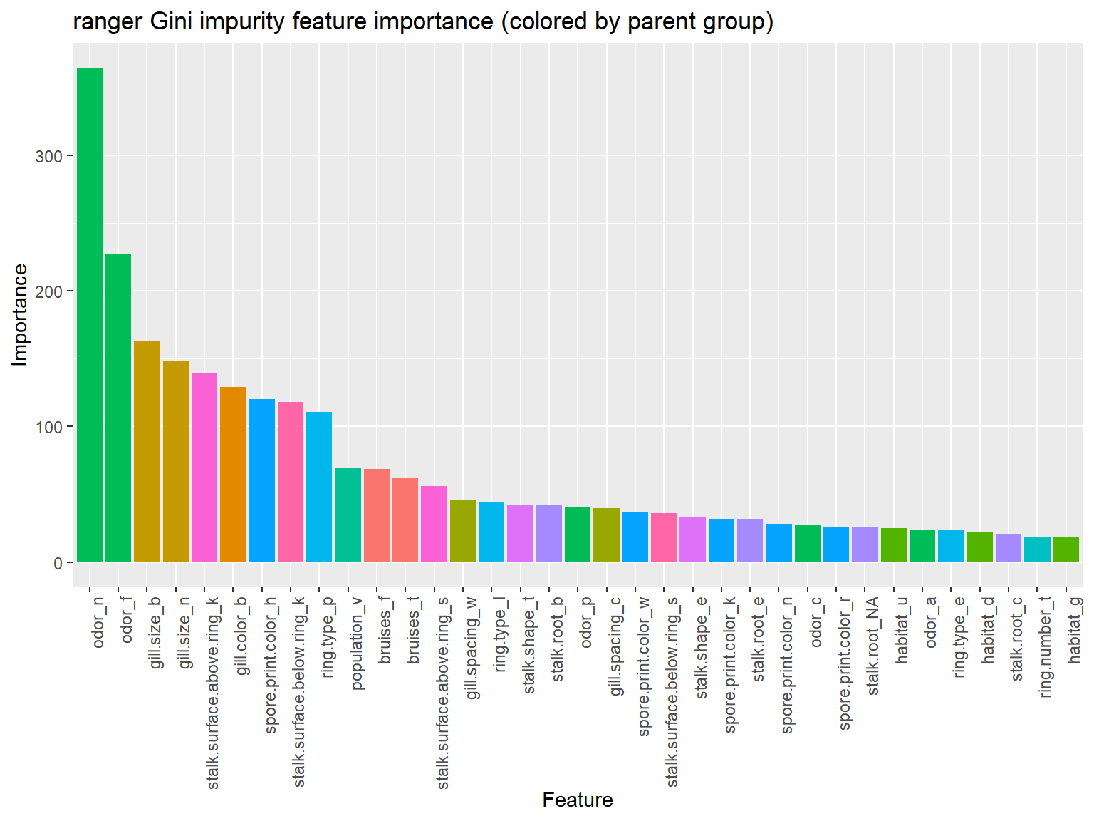
Two odor variables and two gill.size variables are responsible for a large portion of feature importance.
imps.rf %>%
  group_by(featgrp=strsplit(as.character(feature),"_") %>% lapply(`[[`, 1)%>% unlist()) %>%
  summarise(group_importance = sum(importance)) %>%
  ggplot(aes(x=reorder(featgrp,desc(group_importance)), fill=as.factor(featgrp), weight=group_importance)) +
  geom_bar() +
  theme(legend.position="none", axis.text.x = element_text(angle = 90, hjust = 1)) +
  labs(x="Feature Group", y="Importance", title="Total feature importance by group")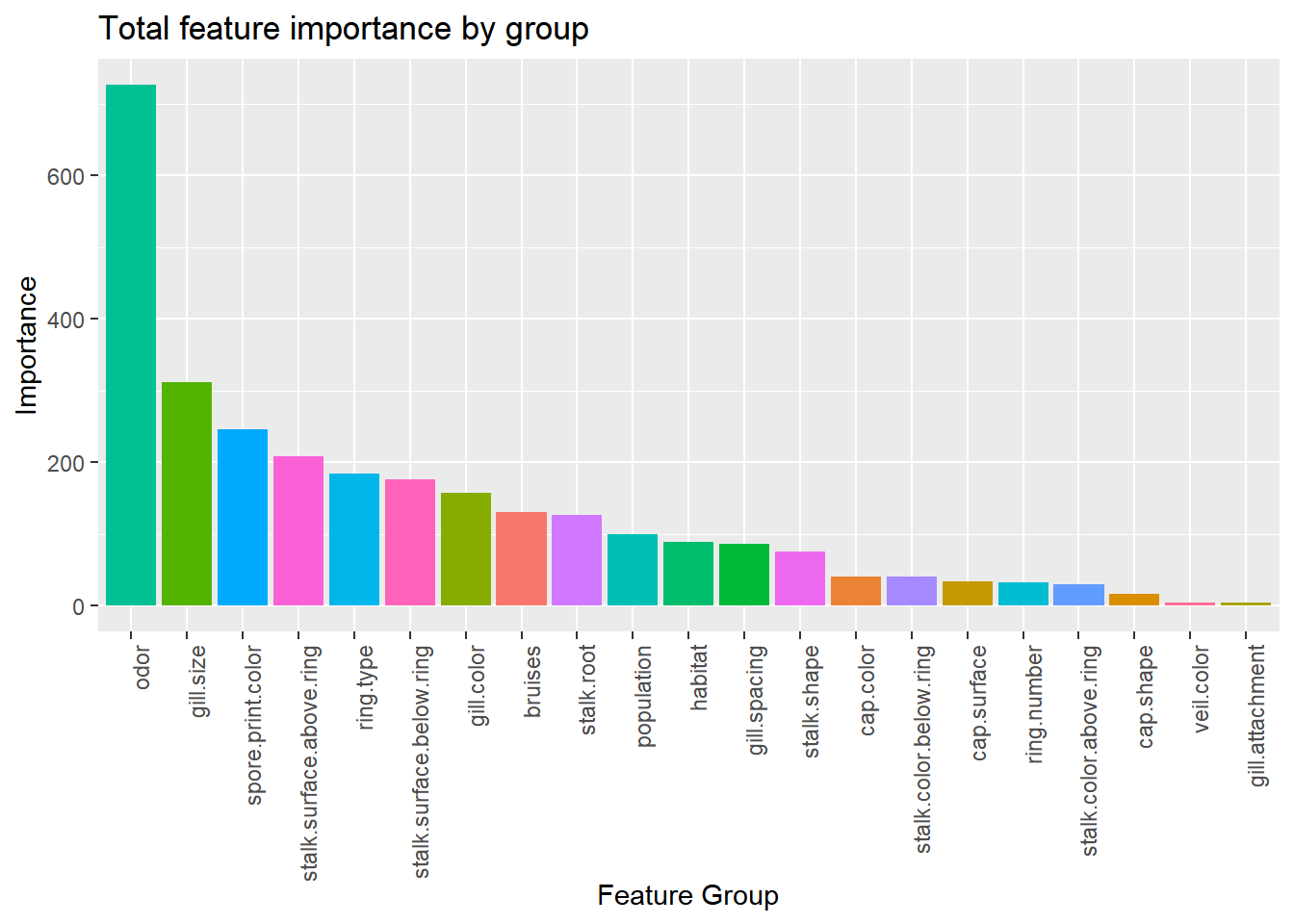
Combining the features by their parent groups gives us a better understanding of how each variable contributes to the model. Odor, by far, is contributing the most in total. If there is any colinearity between predictors and response, these variables would be good place to start the investigation.
XGBoost
library(xgboost)
dtrn <-  as.matrix(subset(agar.train, select = -class))
dtrnlab <- as.matrix(agar.train$class)
dtst <-  as.matrix(subset(agar.test, select = -class))
dtstlab <- as.matrix(agar.test$class)

agar.train.dmx <- xgb.DMatrix(data = dtrn, label=dtrnlab)
agar.test.dmx <- xgb.DMatrix(data = dtst, label=dtstlab)

model.bst <- xgboost(data = agar.train.dmx, max.depth = 2, eta = 1, nthread = 2, nrounds = 2, objective = "binary:logistic")
## [1] train-error:0.045886
## [2] train-error:0.021097preds.bst <- predict(model.bst, agar.test.dmx)
preds.bst.bin <- as.numeric(preds.bst > 0.5)confusionMatrix(as.factor(preds.bst.bin), as.factor(dtstlab))## Confusion Matrix and Statistics
##
## Reference
## Prediction 0 1
## 0 1233 31
## 1 29 1143
##
## Accuracy : 0.9754
## 95% CI : (0.9684, 0.9812)
## No Information Rate : 0.5181
## P-Value [Acc > NIR] : <2e-16
##
## Kappa : 0.9507
##
## Mcnemar's Test P-Value : 0.8973
##
## Sensitivity : 0.9770
## Specificity : 0.9736
## Pos Pred Value : 0.9755
## Neg Pred Value : 0.9753
## Prevalence : 0.5181
## Detection Rate : 0.5062
## Detection Prevalence : 0.5189
## Balanced Accuracy : 0.9753
##
## 'Positive' Class : 0
## dtrain <- xgb.DMatrix(data = train$data, label=train$label)
dtest <- xgb.DMatrix(data = test$data, label=test$label)
bstDMatrix <- xgboost(data = dtrain, max.depth = 2, eta = 1, nthread = 2, nrounds = 2, objective = "binary:logistic")## [1] train-error:0.046522
## [2] train-error:0.022263preds <- predict(bstDMatrix, dtest)
preds.bin <- as.numeric(preds > 0.5)confusionMatrix(as.factor(preds.bin), as.factor(test$label))## Confusion Matrix and Statistics
##
## Reference
## Prediction 0 1
## 0 813 13
## 1 22 763
##
## Accuracy : 0.9783
## 95% CI : (0.9699, 0.9848)
## No Information Rate : 0.5183
## P-Value [Acc > NIR] : <2e-16
##
## Kappa : 0.9565
##
## Mcnemar's Test P-Value : 0.1763
##
## Sensitivity : 0.9737
## Specificity : 0.9832
## Pos Pred Value : 0.9843
## Neg Pred Value : 0.9720
## Prevalence : 0.5183
## Detection Rate : 0.5047
## Detection Prevalence : 0.5127
## Balanced Accuracy : 0.9785
##
## 'Positive' Class : 0
## watchlist <- list(train=dtrain, test=dtest)
bst_lin <- xgb.train(data=dtrain, booster = "gblinear", max.depth=2, nthread = 2, nrounds=2, watchlist=watchlist, eval.metric = "error", eval.metric = "logloss", objective = "binary:logistic")## [1] train-error:0.013511 train-logloss:0.190188 test-error:0.014898 test-logloss:0.194183
## [2] train-error:0.003071 train-logloss:0.082525 test-error:0.002483 test-logloss:0.084925summary(bst_lin)## Length Class Mode
## handle 1 xgb.Booster.handle externalptr
## raw 893 -none- raw
## niter 1 -none- numeric
## evaluation_log 5 data.table list
## call 10 -none- call
## params 7 -none- list
## callbacks 2 -none- list
## feature_names 126 -none- character
## nfeatures 1 -none- numericConclusions
In this notebook we used a Random Forest Classifier and XGBClassifier to attempt to determine if a particular mushroom was toxic when eaten based on its physical characteristics.
The data was converted into the simplest possible numeric representation and a basic one-hot encoding. Using just default hyperparameters, we were able to obtain four perfect classifiers. After double checking our methods, we arrived at the conclusion that certain parts of the dataset maybe have been easier to predict than others.
Ever model had a common feature that it found most importance odor and its one-hot derivations. Tracing down a decision tree from the one-hot RF gives some insight to the process, but it is still a far cry from easily interpretable.
Future work:
Simplifications to the model are certainly possible, feature reduction could provide additional interpretability. PCA could be used to visualize where clustering may be present among the features. There was no parameter tweaking performed at all, this leaves a lot of untapped potential for some improvements to the models. Finally, CatBoost could work wonders with this dataset given that it is only categorical values, it would be interesting to see how well it performs.
References
Code:
https://xgboost.readthedocs.io/en/latest/R-package/xgboostPresentation.html
https://stackoverflow.com/a/20428775/10939610
https://cran.r-project.org/web/packages/ranger/ranger.pdf
https://stackoverflow.com/a/29511387/10939610
Text:
https://archive.ics.uci.edu/ml/datasets/mushroom
https://www.kaggle.com/uciml/mushroom-classification/home
Other:
http://pbpython.com/categorical-encoding.html
http://scikit-learn.org/stable/modules/generated/sklearn.model_selection.StratifiedKFold.html
https://xgboost.readthedocs.io/en/latest/python/python_api.html#xgboost.DMatrix